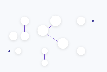
In optimization modeling, understanding dependencies between variables and parameters is fundamental to building accurate and effective models. These relationships define how changes in one factor influence others, forming the backbone of mathematical representations of real-world systems. By identifying and accurately modeling these dependencies, we can ensure that our solutions are both realistic and actionable.
Dependencies are not just mathematical abstractions—they underpin key decisions in fields like supply chain optimization, financial planning, resource allocation and others. Dependencies play a central role in predictive modeling and decision-making systems. For instance, multivariate dependencies are crucial in training machine learning algorithms, while threshold and piecewise relationships are often reflected in decision trees or neural network activations. Mastering these dependencies empowers developers to build models that are robust, adaptable, and insightful, meeting the demands of complex, data-driven environments.
This article explores the main types of relationships in optimization models and provides real-life examples to illustrate their applications.
Proportional Relationships
Proportional dependencies follow the equation y = mx + c, where changes in one variable lead to proportional changes in the other. These relationships are fundamental in linear programming and represent a simple, predictable connection between variables.
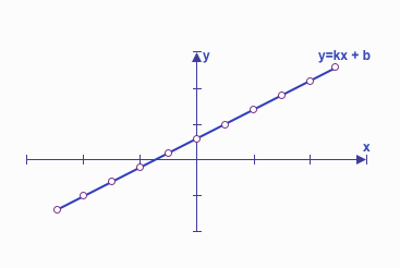
Often, it is required to calculate the sum of a variable over a given period or range. In the context of linear relationships, this summation can provide key insights, such as cumulative totals or accumulated values. For instance, summing a linear function over time is common in scenarios like financial modeling or inventory management.
→ Find out more information about Linear Programs here.
Applications of Proportional Relationships
Examples
ampl model
# Sets
set FACILITIES; # set of facilities
set CUSTOMERS; # set of customers
# Variables
var facility_open{FACILITIES} binary; # 1 if facility i is open, 0 otherwise
var production{FACILITIES, CUSTOMERS} >= 0; # production from facility i to satisfy customer demand
# Parameters
param fixed_cost{FACILITIES} >= 0; # fixed cost of opening facility_open i
param variable_cost{FACILITIES, CUSTOMERS} >= 0; # variable cost of satisfying customer_demand of customer j from facility_open i
param customer_demand{CUSTOMERS} >= 0; # customer_demand of customer j
param facility_capacity{FACILITIES} >= 0; # facility_capacity of facility_open i
# Objective
minimize TotalCost:
sum{i in FACILITIES} fixed_cost[i] * facility_open[i] + # Fixed cost of opening facility i
sum{i in FACILITIES, j in CUSTOMERS} variable_cost[i,j] * production[i,j]; # Variable cost of satisfying customer demand j from facility i
# Constraints
s.t. satisfying_customer_demand{j in CUSTOMERS}:
sum{i in FACILITIES} production[i,j] >= customer_demand[j]; # Satisfy customer demand j
s.t. facility_capacity_limits{i in FACILITIES}:
sum{j in CUSTOMERS} production[i,j] <= facility_capacity[i] * facility_open[i]; # Respect facility capacity limits
s.t. sufficient_production_capacity:
sum{i in FACILITIES} facility_capacity[i]*facility_open[i] >= sum{j in CUSTOMERS} customer_demand[j]; # Ensure there is enough production capacity to satisfy all customer demand
Conditional relationships depend on specific conditions or constraints, often modeled using “if-then” rules or binary variables. These relationships are crucial in capturing decision-based scenarios.
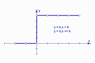
Applications of Conditional Relationships
Manufacturing and Production Scheduling:
Supply Chain and Logistics:
Finance and Investment:
Example (Demand Elasticity: Approach#1)
ampl model
# SETS & PARAMETERS
#Input parameters defining total quantity, cost, price, steps, and demand
para unit_cost >= 0; # Unit cost of the product
param n_step integer > 0; # Number of steps in the piecewise linear price function
param demand {1..n_step} >= 0; # Demand values at each price step
param price {1..n_step} >= 0; # Price values for each demand step
#VARIABLES
#Define decision variables for point selection
var IsSelect {1..n_step} binary; # Binary decision variable: 1 if point is selected, 0 otherwise
#OBJECTIVE
# Maximum total profit based on selected point
maximize TotalProfit:
sum {p in 1..n_step} demand [p] * (price[p] – unit_cost) * IsSelect[p];
#CONSTRAINTS
#Ensure exactly one point is selected
subject to OnePriceSelected:
sum {p in 1..n_step} IsSelect[p] = 1; #Exactly one point is selected
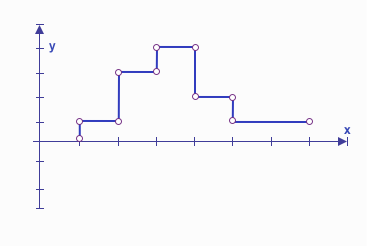
Threshold relationships describe changes in behavior when a variable exceeds or falls below certain critical values. These relationships are common in many fields, such as taxation, pricing, or utilities, where specific thresholds determine changes in behavior or rates.
In “threshold relationships” cases, any value of the independent variable (X-axis) in the corresponding range corresponds to one value of the dependent parameter (Y-axis). In essence, the function “switches” between different ranges of X values, and only one corresponding Y value is used for calculations at any given time, depending on which range X falls into.
Applications of Threshold (Steps) Relationships:
Example (Demand Elasticity: Approach #2)
Below is a fragment of a model for maximizing sales profits by determining the optimal selling price for goods given price elasticity. The decision variables represent the quantity of product sold at each price step and whether the sale occurs at that price. The constraints ensure that sales quantities match demand at each price step and are consistent across adjacent prices.
ampl model
# PARAMETERS
# Input parameters defining total quantity, cost, price steps, and demand
param unit_cost >= 0; # Unit cost of the product
param n_step integer > 0; # Number of steps in the piecewise linear price function
param demand {1..n_step+1} >= 0; # Demand values at each price step
param price {1..n_step+1} >= 0; # Price values for each demand step
# VARIABLES
# Decision variables for managing quantity and selecting price steps
var IsSelect {1..n_step} binary; # Binary decision variable: 1 if point is selected, 0 otherwise
var Quantity_Sold {1..n_step} >= 0, integer; # Quantity sold at each price step
# OBJECTIVE
maximize Total_Profit: # Maximize total revenue from sales while considering costs and constraints
sum{i in 1..n_step} Quantity_Sold[i] * (price[i] – unit_cost);
# CONSTRAINTS
# Ensure logical and physical constraints are met
s.t. OnePriceSelected: # Only one price step can be selected
sum {i in 1..n_step} IsSelect[i] = 1;
s.t. Demand_Upper_Bound {i in 1..n_step-1}:# Quantity sold must align with selected price step
Quantity_Sold[i] <= (demand[i+1] – 0.0001) * IsSelect[i] ;
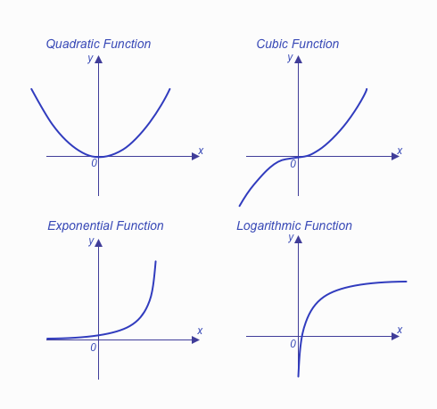
Nonlinear relationships include exponential, quadratic, logarithmic, and other complex forms. These are used to model systems with diminishing returns, growth rates, or other non-proportional dependencies.
Find out more information about Nonlinear Programs here.
Applications of Conditional Relationships:
Example (Hydrothermal Scheduling Problem with Conic Programming):
Hydrothermal scheduling problem involves allocating the total power demand and losses among the hydro and thermal generators in a least-cost way. The scheduling period is typically a few days long. The hydraulic flow constraints and the limits on generator outputs have to be observed in the scheduling problem.
ampl model
param nperiods; ## Number of periods (12 hours long)
set TT := 0..nperiods;
set T := 1..nperiods;
param load {T}; ## load (MW) for the t-th period
param losscof; ## loss coeff for hydro generation / 0.00008 /
param nhours ## number of hours in each period / 12 /
default 12;
param vLU {1..2}; ## storage volume range
param thermalLU {1..2};## steam output range
param hydroUB; ## hydro output upper bound
var cost_sqr{T}>=0; ## quadratic term of the costs
var thermal{T} ## output from the steam thermal plant (MW)
>=thermalLU[1], <=thermalLU[2];
var hydro{T} ## output from the hydro plant (MW)
>=0, <=hydroUB;
var loss{T} >=0; ## total loss (MW)
var q{TT} >=0; ## hydro flow rate in acre-ft per hour
var v{TT} ## reservoir storage volume at the end of t
>=vLU[1], <=vLU[2];
minimize Cost:
1.15*nhours*nperiods * sum {t in T} (500 + 8*thermal[t] + cost_sqr[t]);
s.t. CostPerPeriodSqr {t in T}: ## Extract quadratic terms of the objective
cost_sqr[t] >= 0.0016*(thermal[t] ** 2); ## into a second-order cone
s.t. Loss {t in T}: ## loss calculated as function of hydro output
loss[t] >= losscof*(hydro[t] ** 2); ## another cone
s.t. Demand {t in T}:## demand plus loss must be met from hydro and thermal
thermal[t] + hydro[t] == load[t] + loss[t];
s.t. Flow {t in T}: ## hydraulic continuity equation
v[t] == v[t-1] + (2000 – q[t]) * nhours;
s.t. Dischar {t in T}: ## calculation of hydro discharge
q[t] == 330 +4.97*hydro[t];
In inverse relationships (y = k / x, where y and x are inversely proportional, and k is a constant), one quantity increases as another decreases.
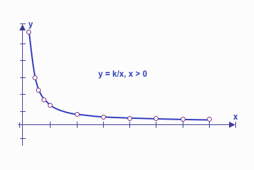
This type of relationship is common in models involving resource allocation, efficiency, or natural laws.
Applications of Inverse Relationships:
Example (Assignment of Workers to Tasks):
The cost of assigning a worker to a task increases as the number of tasks assigned to that worker decreases.
ampl model
# Sets
set WORKERS; # Set of workers
set TASKS; # Set of tasks
# Parameters
param cost {WORKERS, TASKS} >= 0; # Cost of assigning a worker to a task
param max_tasks integer >= 1; # Maximum number of tasks per worker
# Variables
var x {WORKERS, TASKS} binary; # 1 if worker is assigned to task, 0 otherwise
# Objective: Minimize the total cost with inverse relationship scaling
minimize TotalCost:
sum {w in WORKERS, t in TASKS} (cost[w, t] / (1 + sum {t2 in TASKS} x[w, t2])) * x[w, t];
# Constraints
subject to TaskAssignment {t in TASKS}:
sum {w in WORKERS} x[w, t] = 1; # Each task must be assigned to exactly one worker
subject to WorkerLimit {w in WORKERS}:
sum {t in TASKS} x[w, t] <= max_tasks; # Each worker is assigned at most max_tasks tasks
Piecewise relationships occur when a variable’s behavior is described by different functional equations or rules across distinct intervals of another variable. These intervals are often defined by thresholds, boundaries, or ranges. Piecewise relationships are particularly useful when modeling systems with abrupt changes or behaviors that cannot be captured by a single continuous equation.
These relationships are expressed mathematically as:
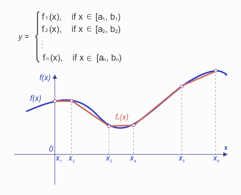
Key Characteristics of Piecewise Relationships:
Why Piecewise Models are Important
Piecewise models simplify and effectively represent real-world scenarios with abrupt or tiered changes. By breaking down complex relationships into manageable segments, they offer:
Find out more information about Piecewise-Linear Programs here.
Applications of Piecewise-Linear Relationships
AMPL Fragment: Tax Brackets
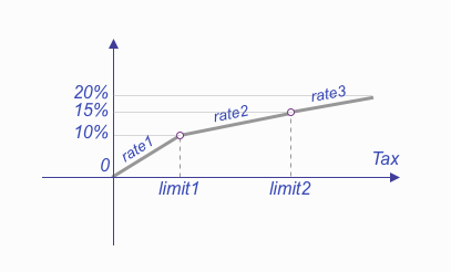
It is necessary to calculate the tax amount taking into account the following rules
Example (Progressive Income Tax Calculation Model):
ampl model
# Parameters
param income; # Total income of the individual 120K USD.
param limit1 >= 0 ; # First tax bracket threshold 50K
param limit2 >= limit1; # Second tax bracket threshold 100K
param rate1 >= 0; # Tax rate (10%) for income <= 50K
param rate2 >= rate2; # Tax rate (15%) for income between 50K and 100K
param rate3 >= rate3; # Tax rate (20%) for income > 100K
# Variable
var Tax >= 0; # Total tax to be calculated
# Constraint: Tax calculation based on income brackets
s.t. TaxCalculation:
tax = <<limit1, limit2; rate1, rate2, rate3>> Tax;
data;
param income := 120000; # Total income of the individual
param limit1 := 50000; # First tax bracket threshold
param limit2 := 100000; # Second tax bracket threshold
param rate1 := 0.10; # Tax rate for income <= 50K
param rate2 := 0.15; # Tax rate for income between 50K and 100K
param rate3 := 0.20; # Tax rate for income > 100K;
Explanation of the Model:
The expression between << and >> describes the piecewise-linear function, and is followed by the name of the variable to which it applies. (You can think of it as ‘‘multiplying’’ Tax, but by a series of coefficients rather than just one.) There are two parts to the expression, a list of breakpoints where the slope of the function changes, and a list of the slopes — which in this case are the cost rates. The lists are separated by a semicolon, and members of each list are separated by commas. Since the first slope applies to values before the first breakpoint, and the last slope to values after the last
breakpoint, the number of slopes must be one more than the number of breakpoints.
Each tax bracket is applied to the corresponding portion of income.
If income is $120,000:
Total tax = $5,000 + $7,500 + $4,000 = $16,500.
This type of relationship is used when it is necessary to calculate values only on the section(s) of the Linear-piecewise function
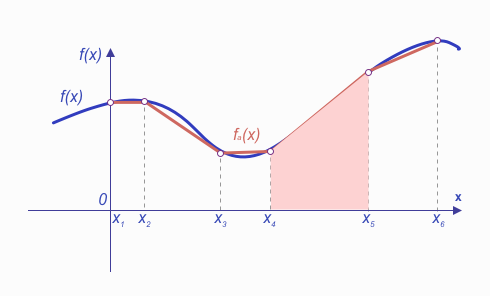
Example (Demand Elasticity: Approach #3):
ampl model
### PARAMETERS
# Input parameters defining total quantity, cost, price steps, and demand
param unit_cost >= 0; # Unit cost of the product
param n_step integer > 0; # Number of steps in the piecewise linear price function
param demand {1..n_step+1} >= 0; # Demand values at each price step
param price {1..n_step+1} >= 0; # Price values for each demand step
### VARIABLES
# Decision variables for managing quantity and selecting price steps
var IsSelect {1..n_step} binary; # Binary decision variable: 1 if point is selected, 0 otherwise
var Quantity_Sold {1..n_step} >= 0, integer; # Quantity sold at each price step
### OBJECTIVE
maximize Total_Profit: # Maximize total revenue from sales while considering costs and constraints
sum {i in 1..n_step}
<<demand[i]; {p in i..i+1} (price[p]– unit_cost)>> Quantity_Sold[i];
# Find more information about the piecewise linear function: https://ampl.com/wp-content/uploads/Chapter-17-Piecewise-Linear-Programs-AMPL-Book.pdf
### CONSTRAINTS
# Ensure logical and physical constraints are met
s.t. OnePriceSelected: # Only one price step can be selected
sum {i in 1..n_step} IsSelect[i] = 1;
s.t. Demand_Upper_Bound {i in 1..n_step–1}:# Quantity sold must align with selected price step
Quantity_Sold[i] <= (demand[i+1] – 0.0001) * IsSelect[i] ;
Find out more information about Piecewise-Linear Programs here.
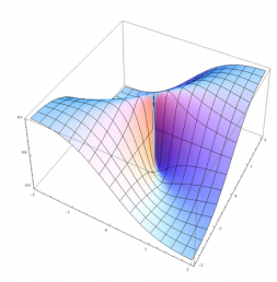
Multivariate relationships describe dependencies where a single output variable (e.g., z) is influenced by multiple input parameters (x,y,…), often represented as:
z = f(x, y, … )
These relationships capture the interactions and combined effects of multiple factors. Unlike simpler relationships, multivariate models account for how variations in several inputs simultaneously impact the outcome, enabling a more holistic understanding of complex systems.
In mathematical optimization, these relationships are crucial for constructing realistic models that consider the combined effects of multiple interdependent factors. Depending on the application, these relationships can take linear, nonlinear, or even stochastic forms.
Applications of Multivariate Relationships
Understanding and accurately modeling dependencies is crucial for developing mathematical optimization models that reflect real-world complexity. From linear to nonlinear and piecewise relationships, each type offers unique insights into how variables interact, enabling models to capture diverse behaviors. Here are key takeaways and best practices for effectively modeling relationships:
By following these practices, developers can construct optimization models that are not only computationally efficient but also aligned with the complexities of real-world systems, paving the way for smarter decisions in fields ranging from logistics and finance to AI-driven analytics.