Extra material: Luenberger’s Investment Wheel

Extra material: Luenberger’s Investment Wheel#

# install dependencies and select solver
%pip install -q amplpy numpy pandas matplotlib ipywidgets

SOLVER_CONIC = "mosek"  ## ipopt, mosek, knitro

from amplpy import AMPL, ampl_notebook

ampl = ampl_notebook(
    modules=["coin", "mosek"],  # modules to install
    license_uuid="default",  # license to use
)  # instantiate AMPL object and register notebook magics

Problem statement#

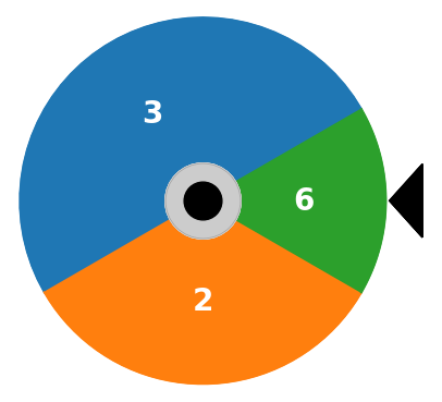
David Luenberger presents an “investment wheel” in Chapter 18 of his book Investment Science. The wheel is divided into sectors, each marked with a number. An investor places wagers on one or more sectors before spinning the wheel. When the wheel stops, the investor receives a payout equal to the wager times the number appearing next to the marker. The wagers on all other sectors are lost. The game is repeated indefinitely.

Given an initial wealth \(W_0\), what is your investing strategy for repeated plays of the game?

Is there an investing strategy that almost surely grows?
What is the mean return for each spin of the wheel?

# specify the investment wheel
wheel = {
    "A": {"p": 1 / 2, "b": 3},
    "B": {"p": 1 / 3, "b": 2},
    "C": {"p": 1 / 6, "b": 6},
}

Simulation#

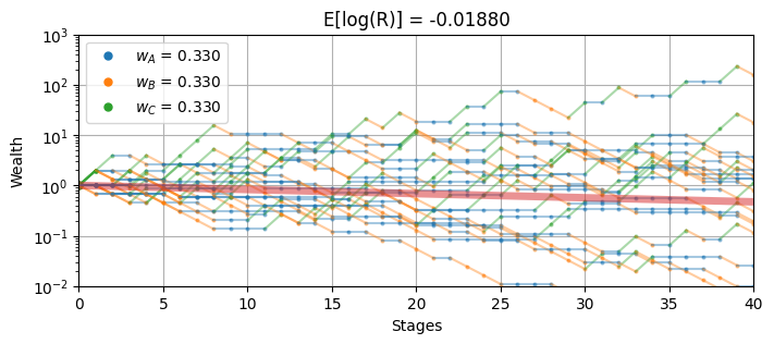
The following cell provides an interactive simulation of the investment wheel. The weighting parameters \(w_A\), \(w_B\), and \(w_C\) represent the fraction of the investor’s current stake that is wagered on sectors \(A\), \(B\), and \(C\), respectively. Experiment with the simulation to find weights that produce an acceptable compromise between long term return and risk.

import numpy as np
import matplotlib.pyplot as plt
import bisect

import ipywidgets as widgets


def wheel_sim(w, T, N):
    # set of wheel sectors
    S = list(wheel.keys())

    # odds, probability, and quantiles
    b = {s: wheel[s]["b"] for s in S}
    p = {s: wheel[s]["p"] for s in S}
    q = np.cumsum(list(p.values()))

    # gross return for each sector
    R = {s: 1 + w[s] * b[s] - sum(w.values()) for s in S}

    # set up plot and colors
    _, ax = plt.subplots(1, 1, figsize=(8, 3))
    colors = {s: ax.semilogy(0, 1, ".", ms=10)[0].get_color() for s in S}

    # repeat the simulation N times
    for _ in range(N):
        wealth = 1.0
        for k in range(T):
            # spin the wheel
            spin = np.random.uniform()
            s = S[bisect.bisect_left(q, spin)]
            wealth_next = wealth * R[s]

            # add to plot
            ax.semilogy([k, k + 1], [wealth, wealth_next], c=colors[s], alpha=0.4)
            ax.semilogy(k + 1, wealth_next, ".", ms=4, c=colors[s], alpha=0.4)
            wealth = wealth_next

    # compute expected log return
    ElogR = sum(p[s] * np.log(R[s]) for s in S)
    ax.plot(np.exp(ElogR * np.linspace(0, T, T + 1)), lw=5, alpha=0.5)
    ax.set_title(f"E[log(R)] = {ElogR:0.5f}")
    ax.legend([f"$w_{s}$ = {w[s]:0.3f}" for s in S])
    ax.set_xlim(0, T)
    ax.set_ylim(0.01, 1000.0)
    ax.set_ylabel("Wealth")
    ax.set_xlabel("Stages")
    ax.grid(True)
    return ax


wheel_sim({"A": 0.33, "B": 0.33, "C": 0.33}, 40, 20)


@widgets.interact_manual(
    wA=widgets.FloatSlider(min=0.0, max=1.0, step=0.01, value=0.333),
    wB=widgets.FloatSlider(min=0.0, max=1.0, step=0.01, value=0.333),
    wC=widgets.FloatSlider(min=0.0, max=1.0, step=0.01, value=0.333),
)
def wheel_interact1(wA, wB, wC):
    w = {"A": wA, "B": wB, "C": wC}
    wheel_sim(w, 40, 20)

../../_images/21e1e0fd775f9e57a4107a36dc45b8e77598aa30536559701b7f661e5a7075b3.png

Modeling#

The investment wheel is an example of a game with \(n=3\) outcomes. Each outcome \(n\) offers payout \(b_n\) that occurs with probability \(p_n\) as given in the following table.

Outcome	Probability \(p_n\)	Odds \(b_n\)
A	1/2	3
B	1/3	2
C	1/6	6

If a \(w_n\) of current wealth is wagered on each outcome \(n\), then the gross returns \(R_n\) are given in the following table.

Outcome	Probability \(p_n\)	Gross Returns \(R_n\)
A	1/2	1 + 2\(w_A\) - \(w_B\) - \(w_C\)
B	1/3	1 - \(w_A\) + \(w_B\) - \(w_C\)
C	1/6	1 - \(w_A\) - \(w_B\) + 5\(w_C\)

Following the same analysis used for the Kelly criterion, the optimization problem is to maximize expected log return

\[\begin{split} \begin{align} \max_{w \geq 0}\quad & \sum_{n\in N} p_n \log(R_n) \\ \text{s.t.}\quad \\ & \sum_{n\in N} w_n \leq 1 \\ & R_n = 1 + b_n w_n - \sum_{n\in N} w_n & \forall n\in N \\ \end{align} \end{split}\]

The objective function can be reformulated using exponential cones to a conic optimization problem.

\[\begin{split} \begin{align} \max_{w\geq 0}\quad & \sum_{n\in N} p_n q_n \\ \text{s.t.}\quad \\ & \sum_{n\in N} w_n \leq 1 \\ & R_n = 1 + b_n w_n - \sum_{n\in N} w_n & \forall n\in N \\ & (R_n, 1, q_n) \in K_{exp} & \forall n \in N \\ \end{align} \end{split}\]

The solution of this optimization problem is shown below.

%%writefile wheel.mod

set S;

param p{S};
param b{S};

# decision variables
var w{S} >= 0;
var q{S};
    
# objective
maximize ElogR:       sum {s in S} p[s]*q[s];
    
# expression for returns
var R{s in S} = 1 + b[s]*w[s] - sum {t in S} w[t];
    
# constraints
s.t. SumW:            sum {s in S} w[s] <= 1;
s.t. Conic{s in S}:   R[s] >= exp(q[s]);

Overwriting wheel.mod

def wheel_model(wheel):
    ampl = AMPL()
    ampl.read("wheel.mod")

    ampl.set["S"] = list(wheel.keys())
    ampl.param["p"] = {s: wheel[s]["p"] for s in wheel.keys()}
    ampl.param["b"] = {s: wheel[s]["b"] for s in wheel.keys()}

    ampl.solve(solver=SOLVER_CONIC)
    assert ampl.solve_result == "solved", ampl.solve_result

    return ampl


m = wheel_model(wheel)
w = m.get_variable("w").to_dict()

print(f"Expected Log Return = {m.get_objective('ElogR').value(): 0.5f}\n")
for s in wheel.keys():
    print(
        f"Sector {s}:  p = {wheel[s]['p']:0.3f}   b = {wheel[s]['b']:0.2f}   w = {w[s]:0.3f}"
    )

wheel_sim(w, 40, 20)

MOSEK 10.0.43: MOSEK 10.0.43: optimal; objective 0.06757751812
0 simplex iterations
8 barrier iterations
Expected Log Return =  0.06758

Sector A:  p = 0.500   b = 3.00   w = 0.423
Sector B:  p = 0.333   b = 2.00   w = 0.218
Sector C:  p = 0.167   b = 6.00   w = 0.128

../../_images/3b5827c7508346fdbfafc9a4e9bf98d8ce366595232c043d74f0ae16145912ed.png

Adding risk aversion#

The Kelly criterion has favorable properties for the long term investor, but suffers from a significant chance of “drawdown” where the investor’s wealth drops below the initial value, sometimes without recovering for a long period of time. For this reason, investors normally augment the Kelly criterion with some sort of strategy for risk aversion.

Here we follow the analysis of Busseti, Ryu, and Boyd (2016) for risk-constrained Kelly gambling. Consider a constraint

\[\mathbb{E}[R^{-\lambda}] \leq 1\]

where \(\lambda\) is a risk aversion parameter. For the case of \(N\) discrete outcomes

\[\sum_{n\in N} p_n R_n^{-\lambda} \leq 1\]

The case \(\lambda=0\) is always satisfied and imposes no further restrictions on an optimization problem. This is this case of no risk-aversion. If \(\lambda > 0\) then outcomes with gross returns less than one are penalized. As \(\lambda \rightarrow \infty\) no solutions are admissible with a gross return less than one. In that case a feasible solution \(w_n = 0\) for all \(n\in N\) always exists, and there may other non-trivial solutions as well.

Replacing each term with an exponential

\[\sum_{n\in N} e^{\log(p_1) - \lambda\log(R_1)} \leq 1\]

Introducing \(u_n \geq e^{\log(p_n) - \lambda q_n}\) using the \(q_n\) defined above, we get

\[\begin{split} \begin{align} \sum_{n\in N} u_n & \leq 1 \\ (u_n, 1, \log(p_n) - \lambda q_n) & \in K_{exp} & \forall n\in N \\ \end{align} \end{split}\]

The risk-constrained investment wheel is now

\[\begin{split} \begin{align} \max_{w\geq 0}\quad & \sum_{n\in N} p_n q_n \\ \text{s.t.}\quad \\ & \sum_{n\in N} w_n \leq 1 \\ &\sum_{n\in N} u_n \leq 1 \\ & R_n = 1 + b_n w_n - \sum_{n\in N} w_n & \forall n\in N \\ & (R_n, 1, q_n) \in K_{exp} & \forall n \in N \\ & (u_n, 1, \log(p_n) - \lambda q_n) \in K_{exp} & \forall n\in N \\ \end{align} \end{split}\]

The following cell creates a risk-constrained model of the investment wheel.

%%writefile wheel_risk_averse.mod

set S;

param p{S};
param b{S};
param lambd;

# decision variables
var w{S} >= 0;
var q{S};
    
# objective
maximize ElogR:       sum {s in S} p[s]*q[s];
    
# expression for returns
var R{s in S} = 1 + b[s]*w[s] - sum {t in S} w[t];
    
# constraints
s.t. SumW:            sum {s in S} w[s] <= 1;
s.t. Conic{s in S}:   R[s] >= exp(q[s]);

# risk constraints
var u{S};
s.t. SumU:            sum {s in S} u[s] <= 1;
s.t. Risk{s in S}:    u[s] >= exp(log(p[s]) - lambd*q[s]);

Overwriting wheel_risk_averse.mod

def wheel_rc_model(wheel, lambd=0):
    ampl = AMPL()
    ampl.read("wheel_risk_averse.mod")

    ampl.set["S"] = list(wheel.keys())
    ampl.param["p"] = {s: wheel[s]["p"] for s in wheel.keys()}
    ampl.param["b"] = {s: wheel[s]["b"] for s in wheel.keys()}
    ampl.param["lambd"] = lambd

    ampl.solve(solver=SOLVER_CONIC)
    assert ampl.solve_result == "solved", ampl.solve_result

    return (
        ampl.get_variable("w").to_dict(),
        ampl.get_objective("ElogR").value(),
    )


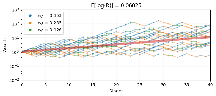
lambd = 2
w, obj = wheel_rc_model(wheel, lambd)

print(f"Risk-aversion lambda = {lambd:0.3f}")
print(f"Expected Log Gross Return = {obj:0.5f}\n")
for s in wheel.keys():
    print(
        f"Sector {s}:  p = {wheel[s]['p']:0.4f}   b = {wheel[s]['b']:0.2f}   w = {w[s]:0.5f}"
    )

wheel_sim(w, 40, 20)

MOSEK 10.0.43: MOSEK 10.0.43: optimal; objective 0.06024886223
0 simplex iterations
10 barrier iterations
Risk-aversion lambda = 2.000
Expected Log Gross Return = 0.06025

Sector A:  p = 0.5000   b = 3.00   w = 0.36330
Sector B:  p = 0.3333   b = 2.00   w = 0.26549
Sector C:  p = 0.1667   b = 6.00   w = 0.12576

<Axes: title={'center': 'E[log(R)] = 0.06025'}, xlabel='Stages', ylabel='Wealth'>

../../_images/bf8628bc8206090a3943e317ee825ed236062f1607db1664db0aec63ddcd28e1.png

@widgets.interact_manual(
    lambd=widgets.FloatSlider(min=0.0, max=20.0, step=0.1, value=2),
)
def wheel_interact2(lambd):
    w, _ = wheel_rc_model(wheel, lambd)
    wheel_sim(w, 40, 20)

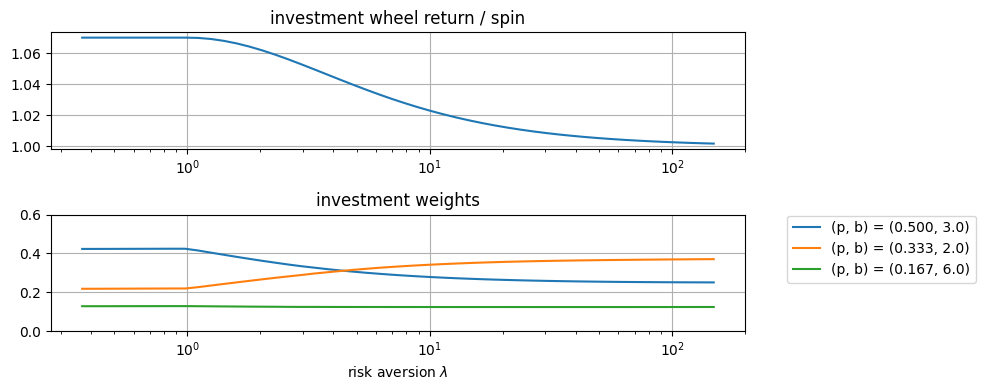
How does risk aversion change the solution?#

The following cell demonstrates the effect of increasing the risk aversion parameter \(\lambda\).

import matplotlib.pyplot as plt
import numpy as np

fig, ax = plt.subplots(2, 1, figsize=(10, 4))

v = np.linspace(-1, 5)
lambd = np.exp(v)
results = [wheel_rc_model(wheel, _) for _ in lambd]

ax[0].semilogx(lambd, [np.exp(obj) for _, obj in results])
ax[0].set_title("investment wheel return / spin")
ax[0].grid(True)

ax[1].semilogx(lambd, [[w[s] for s in wheel.keys()] for w, _ in results])
ax[1].set_title("investment weights")
ax[1].set_xlabel("risk aversion $\lambda$")
ax[1].legend(
    [f"(p, b) = ({wheel[s]['p']:0.3f}, {wheel[s]['b']:0.1f})" for s in wheel.keys()],
    bbox_to_anchor=(1.05, 1.05),
)
ax[1].grid(True)
ax[1].set_ylim(0, 0.6)

fig.tight_layout()

MOSEK 10.0.43: MOSEK 10.0.43: optimal; objective 0.067577517
0 simplex iterations
8 barrier iterations
MOSEK 10.0.43: MOSEK 10.0.43: optimal; objective 0.06757751809
0 simplex iterations
9 barrier iterations
MOSEK 10.0.43: MOSEK 10.0.43: optimal; objective 0.0675775181
0 simplex iterations
9 barrier iterations
MOSEK 10.0.43: MOSEK 10.0.43: optimal; objective 0.06757751964
0 simplex iterations
9 barrier iterations
MOSEK 10.0.43: MOSEK 10.0.43: optimal; objective 0.06757751754
0 simplex iterations
10 barrier iterations
MOSEK 10.0.43: MOSEK 10.0.43: optimal; objective 0.0675775172
0 simplex iterations
11 barrier iterations
MOSEK 10.0.43: MOSEK 10.0.43: optimal; objective 0.06757751754
0 simplex iterations
9 barrier iterations
MOSEK 10.0.43: MOSEK 10.0.43: optimal; objective 0.06757751218
0 simplex iterations
9 barrier iterations
MOSEK 10.0.43: MOSEK 10.0.43: optimal; objective 0.06757751966
0 simplex iterations
12 barrier iterations
MOSEK 10.0.43: MOSEK 10.0.43: optimal; objective 0.06740662006
0 simplex iterations
10 barrier iterations
MOSEK 10.0.43: MOSEK 10.0.43: optimal; objective 0.06675561718
0 simplex iterations
10 barrier iterations
MOSEK 10.0.43: MOSEK 10.0.43: optimal; objective 0.06563611352
0 simplex iterations
10 barrier iterations
MOSEK 10.0.43: MOSEK 10.0.43: optimal; objective 0.06407923979
0 simplex iterations
10 barrier iterations
MOSEK 10.0.43: MOSEK 10.0.43: optimal; objective 0.06212703771
0 simplex iterations
10 barrier iterations
MOSEK 10.0.43: MOSEK 10.0.43: optimal; objective 0.05983012807
0 simplex iterations
10 barrier iterations
MOSEK 10.0.43: MOSEK 10.0.43: optimal; objective 0.05724509196
0 simplex iterations
10 barrier iterations
MOSEK 10.0.43: MOSEK 10.0.43: optimal; objective 0.05443169986
0 simplex iterations
10 barrier iterations
MOSEK 10.0.43: MOSEK 10.0.43: optimal; objective 0.05145030888
0 simplex iterations
10 barrier iterations
MOSEK 10.0.43: MOSEK 10.0.43: optimal; objective 0.0483595141
0 simplex iterations
11 barrier iterations
MOSEK 10.0.43: MOSEK 10.0.43: optimal; objective 0.04521417102
0 simplex iterations
10 barrier iterations
MOSEK 10.0.43: MOSEK 10.0.43: optimal; objective 0.04206396075
0 simplex iterations
10 barrier iterations
MOSEK 10.0.43: MOSEK 10.0.43: optimal; objective 0.03895235786
0 simplex iterations
10 barrier iterations
MOSEK 10.0.43: MOSEK 10.0.43: optimal; objective 0.0359161105
0 simplex iterations
10 barrier iterations
MOSEK 10.0.43: MOSEK 10.0.43: optimal; objective 0.03298511723
0 simplex iterations
10 barrier iterations
MOSEK 10.0.43: MOSEK 10.0.43: optimal; objective 0.03018262271
0 simplex iterations
9 barrier iterations
MOSEK 10.0.43: MOSEK 10.0.43: optimal; objective 0.02752566085
0 simplex iterations
10 barrier iterations
MOSEK 10.0.43: MOSEK 10.0.43: optimal; objective 0.02502566272
0 simplex iterations
10 barrier iterations
MOSEK 10.0.43: MOSEK 10.0.43: optimal; objective 0.02268918883
0 simplex iterations
10 barrier iterations
MOSEK 10.0.43: MOSEK 10.0.43: optimal; objective 0.0205186608
0 simplex iterations
10 barrier iterations
MOSEK 10.0.43: MOSEK 10.0.43: optimal; objective 0.01851310984
0 simplex iterations
10 barrier iterations
MOSEK 10.0.43: MOSEK 10.0.43: optimal; objective 0.01666886968
0 simplex iterations
10 barrier iterations
MOSEK 10.0.43: MOSEK 10.0.43: optimal; objective 0.01498021386
0 simplex iterations
10 barrier iterations
MOSEK 10.0.43: MOSEK 10.0.43: optimal; objective 0.01343991471
0 simplex iterations
11 barrier iterations
MOSEK 10.0.43: MOSEK 10.0.43: optimal; objective 0.01203970957
0 simplex iterations
11 barrier iterations
MOSEK 10.0.43: MOSEK 10.0.43: optimal; objective 0.01077071324
0 simplex iterations
11 barrier iterations
MOSEK 10.0.43: MOSEK 10.0.43: optimal; objective 0.009623732846
0 simplex iterations
11 barrier iterations
MOSEK 10.0.43: MOSEK 10.0.43: optimal; objective 0.008589525912
0 simplex iterations
11 barrier iterations
MOSEK 10.0.43: MOSEK 10.0.43: optimal; objective 0.00765899591
0 simplex iterations
11 barrier iterations
MOSEK 10.0.43: MOSEK 10.0.43: optimal; objective 0.006823340138
0 simplex iterations
11 barrier iterations
MOSEK 10.0.43: MOSEK 10.0.43: optimal; objective 0.006074151751
0 simplex iterations
11 barrier iterations
MOSEK 10.0.43: MOSEK 10.0.43: optimal; objective 0.005403490806
0 simplex iterations
11 barrier iterations
MOSEK 10.0.43: MOSEK 10.0.43: optimal; objective 0.00480392626
0 simplex iterations
11 barrier iterations
MOSEK 10.0.43: MOSEK 10.0.43: optimal; objective 0.004268555008
0 simplex iterations
11 barrier iterations
MOSEK 10.0.43: MOSEK 10.0.43: optimal; objective 0.003791005462
0 simplex iterations
11 barrier iterations
MOSEK 10.0.43: MOSEK 10.0.43: optimal; objective 0.003365428946
0 simplex iterations
11 barrier iterations
MOSEK 10.0.43: MOSEK 10.0.43: optimal; objective 0.002986479423
0 simplex iterations
10 barrier iterations
MOSEK 10.0.43: MOSEK 10.0.43: optimal; objective 0.002649298922
0 simplex iterations
10 barrier iterations
MOSEK 10.0.43: MOSEK 10.0.43: optimal; objective 0.002349479711
0 simplex iterations
10 barrier iterations
MOSEK 10.0.43: MOSEK 10.0.43: optimal; objective 0.002083031114
0 simplex iterations
10 barrier iterations
MOSEK 10.0.43: MOSEK 10.0.43: optimal; objective 0.001846361945
0 simplex iterations
10 barrier iterations

../../_images/02d843f1a25e7f8519593401b29162d505f04599fcab4a36ac407b137b0aeba3.png

Exercises#

Is there a deterministic investment strategy for the investment wheel?. That is, is there investment strategy that provides a fixed return regardless of the outcome of the spin? Set up and solve a model to find that strategy.
Find the variance in the outcome of the wheel, and plot the variance as a function of the risk aversion parameter \(\lambda\). What is the relationship of variance and \(\lambda\) in the limit as \(\lambda \rightarrow 0\)? See the paper by Busseti, E., Ryu, E. K., & Boyd, S. (2016) for ideas on how to perform this analysis.

Bibliographic Notes#

The Kelly Criterion has been included in many tutorial introductions to finance and probability, and the subject of popular accounts.

Poundstone, W. (2010). Fortune’s formula: The untold story of the scientific betting system that beat the casinos and Wall Street. Hill and Wang. https://www.onlinecasinoground.nl/wp-content/uploads/2020/10/Fortunes-Formula-boek-van-William-Poundstone-oa-Kelly-Criterion.pdf

Thorp, E. O. (2017). A man for all markets: From Las Vegas to wall street, how i beat the dealer and the market. Random House.

Thorp, E. O. (2008). The Kelly criterion in blackjack sports betting, and the stock market. In Handbook of asset and liability management (pp. 385-428). North-Holland. https://www.palmislandtraders.com/econ136/thorpe_kelly_crit.pdf

MacLean, L. C., Thorp, E. O., & Ziemba, W. T. (2010). Good and bad properties of the Kelly criterion. Risk, 20(2), 1. https://www.stat.berkeley.edu/~aldous/157/Papers/Good_Bad_Kelly.pdf

MacLean, L. C., Thorp, E. O., & Ziemba, W. T. (2011). The Kelly capital growth investment criterion: Theory and practice (Vol. 3). world scientific. https://www.worldscientific.com/worldscibooks/10.1142/7598#t=aboutBook

https://en.wikipedia.org/wiki/Kelly_criterion

Luenberger’s investment wheel is

Luenberger, D. (2009). Investment science: International edition. OUP Catalogue. https://global.oup.com/ushe/product/investment-science-9780199740086

The utility of conic optimization to solve problems involving log growth is more recent. Here are some representative papers.

Cajas, D. (2021). Kelly Portfolio Optimization: A Disciplined Convex Programming Framework. Available at SSRN 3833617. https://papers.ssrn.com/sol3/papers.cfm?abstract_id=3833617

Busseti, E., Ryu, E. K., & Boyd, S. (2016). Risk-constrained Kelly gambling. The Journal of Investing, 25(3), 118-134. https://arxiv.org/pdf/1603.06183.pdf

Fu, A., Narasimhan, B., & Boyd, S. (2017). CVXR: An R package for disciplined convex optimization. arXiv preprint arXiv:1711.07582. https://arxiv.org/abs/1711.07582

Sun, Q., & Boyd, S. (2018). Distributional robust Kelly gambling. arXiv preprint arXiv: 1812.10371. https://web.stanford.edu/~boyd/papers/pdf/robust_kelly.pdf

The recent work by CH Hsieh extends these concepts in important ways for real-world implementation.

Hsieh, C. H. (2022). On Solving Robust Log-Optimal Portfolio: A Supporting Hyperplane Approximation Approach. arXiv preprint arXiv:2202.03858. https://arxiv.org/pdf/2202.03858