Enhanced Sector ETF Portfolio Optimization with Multiple Strategies in Python with AMPL#
![]()
![]()


![]()

Description: This notebook compares multiple portfolio optimization strategies for invesment in Sector ETFs
Tags: finance, portfolio-optimization
Notebook author: Mukeshwaran Baskaran <mukesh96official@gmail.com>
Introduction#
This notebook helps you make better investment decisions by optimizing a portfolio of sector ETFS. It uses different portfolio optimisation strategies to decide how much of your money should go into each ETF. The goal is to balance risk and potential gains. The notebook shows you how different strategies perform over time and helps you compare their results. AMPL helps to perform this optimisation.
# Install dependencies
%pip install amplpy yfinance seaborn matplotlib pandas numpy -q
# Google Colab & Kaggle integration
from amplpy import AMPL, ampl_notebook

ampl = ampl_notebook(
    modules=["gurobi"],  # modules to install
    license_uuid="default",  # license to use
)  # instantiate AMPL object and register magics
Implementation#
Import libraries#
import yfinance as yf
import pandas as pd
import numpy as np
import matplotlib.pyplot as plt
import seaborn as sns
Define constants#
# Define sector ETFs
SECTOR_ETFS = [
    "XLK",  # Technology
    "XLF",  # Financials
    "XLV",  # Healthcare
    "XLE",  # Energy
    "XLY",  # Consumer Discretionary
    "XLC",  # Communication Services
    "VWO",  # Vanguard Emerging Markets (Global Exposure)
    "BND",  # Vanguard Total Bond Market ETF (Fixed Income)
    "GLD",  # SPDR Gold Shares (Commodity, Gold)
]

START_DATE = "2007-01-01"
END_DATE = "2020-01-01"
Download historical data for sector ETFs#
def fetch_sector_data(tickers, start_date, end_date):
    """Fetch historical data for given tickers."""
    data = yf.download(tickers, start=start_date, end=end_date)["Close"]
    if data.empty:
        raise ValueError("No data fetched. Check tickers and date range.")
    return data
Calculate returns and covariance matrix#
def calculate_statistics(data):
    """Calculate daily returns and covariance matrix."""
    returns = data.pct_change().dropna()
    cov_matrix = returns.cov().values
    mean_returns = returns.mean().values
    return returns, cov_matrix, mean_returns
Minimum Variance Optimization using AMPL#
def minimum_variance_optimization(tickers, cov_matrix):
    """Perform minimum variance optimization."""
    ampl = AMPL()
    ampl.eval(
        r"""
        set A ordered;  # Set of assets
        param S{A, A};  # Covariance matrix
        var w{A} >= 0 <= 1;  # Portfolio weights

        minimize min_variance:
            sum {i in A, j in A} w[i] * S[i, j] * w[j];  # Objective: minimize variance

        s.t. portfolio_weights:
            sum {i in A} w[i] = 1;  # Constraint: weights sum to 1
    """
    )
    ampl.set["A"] = tickers
    ampl.param["S"] = pd.DataFrame(cov_matrix, index=tickers, columns=tickers)
    ampl.solve(solver="gurobi", mp_options="outlev=1")
    assert ampl.solve_result == "solved", ampl.solve_result
    return pd.Series(ampl.var["w"].to_dict())
Markowitz (Mean-Variance) Optimization using AMPL#
def markowitz_optimization(tickers, cov_matrix, mean_returns, risk_tolerance):
    """Perform Markowitz mean-variance optimization."""
    ampl = AMPL()
    ampl.eval(
        r"""
        set A ordered;  # Set of assets
        param S{A, A};  # Covariance matrix
        param mu{A};    # Expected returns
        param gamma;    # Risk tolerance
        var w{A} >= 0 <= 1;  # Portfolio weights

        maximize expected_return:
            sum {i in A} mu[i] * w[i];  # Objective: maximize expected return

        s.t. portfolio_weights:
            sum {i in A} w[i] = 1;  # Constraint: weights sum to 1

        s.t. risk_constraint:
            sum {i in A, j in A} w[i] * S[i, j] * w[j] <= gamma;  # Risk constraint
    """
    )
    ampl.set["A"] = tickers
    ampl.param["S"] = pd.DataFrame(cov_matrix, index=tickers, columns=tickers)
    ampl.param["mu"] = pd.Series(mean_returns, index=tickers)
    ampl.param["gamma"] = risk_tolerance
    ampl.solve(solver="gurobi", mp_options="outlev=1")
    assert ampl.solve_result == "solved", ampl.solve_result
    return pd.Series(ampl.var["w"].to_dict())
Equal-Weighted Portfolio#
def equal_weighted_portfolio(tickers):
    """Equal-weighted portfolio."""
    n_assets = len(tickers)
    return pd.Series(np.ones(n_assets) / n_assets, index=tickers)
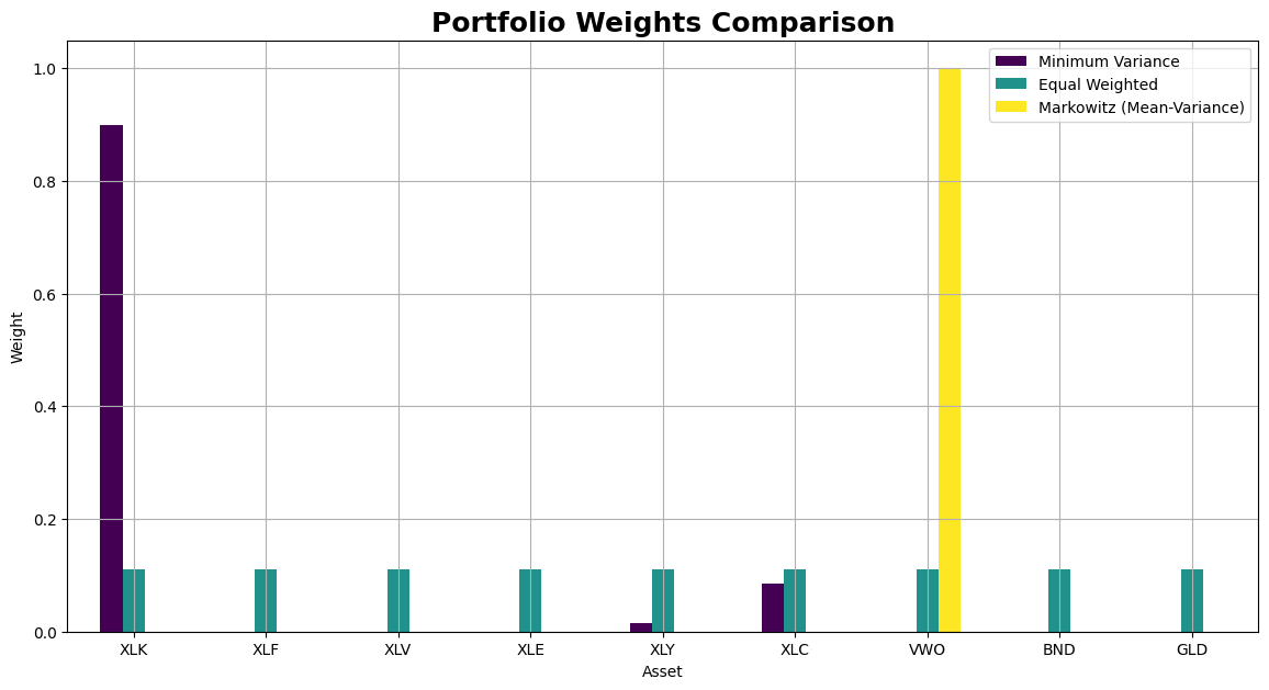
Plot portfolio weights comparison#
def plot_weights_comparison(weights_dict):
    """Plot comparison of portfolio weights across strategies."""
    weights_df = pd.DataFrame(weights_dict)
    weights_df.plot(kind="bar", figsize=(14, 7), colormap="viridis")
    plt.title("Portfolio Weights Comparison", fontsize=18, fontweight="bold")
    plt.xlabel("Asset")
    plt.ylabel("Weight")
    plt.xticks(rotation=0)
    plt.grid(True)
    plt.show()
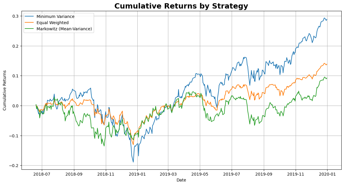
Plot cumulative returns#
def plot_cumulative_returns(returns, weights_dict):
    """Plot cumulative returns for each strategy."""
    plt.figure(figsize=(14, 7))
    for strategy, weights in weights_dict.items():
        portfolio_returns = returns.dot(weights)
        cumulative_returns = (1 + portfolio_returns).cumprod() - 1
        plt.plot(cumulative_returns, label=strategy)
    plt.title("Cumulative Returns by Strategy", fontsize=18, fontweight="bold")
    plt.xlabel("Date")
    plt.ylabel("Cumulative Returns")
    plt.legend()
    plt.grid(True)
    plt.show()
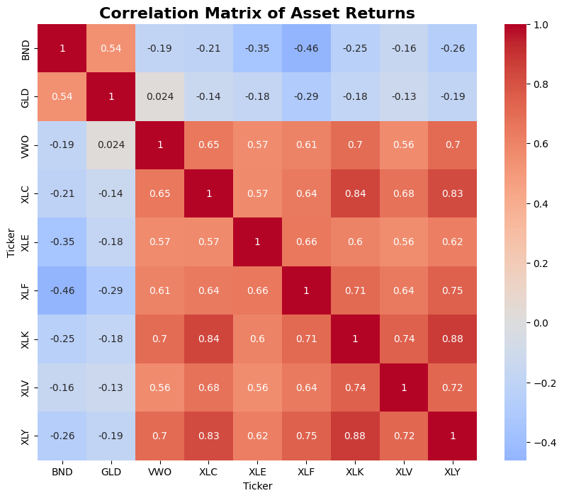
Plot correlation matrix#
def plot_correlation_matrix(returns):
    """Plot correlation matrix of asset returns."""
    plt.figure(figsize=(10, 8))
    sns.heatmap(returns.corr(), annot=True, cmap="coolwarm", center=0)
    plt.title("Correlation Matrix of Asset Returns", fontsize=16, fontweight="bold")
    plt.show()
Calculate portfolio performance metrics#
def calculate_performance_metrics(returns, weights, risk_free_rate=0):
    """Calculate portfolio performance metrics."""
    portfolio_returns = returns.dot(weights)
    cumulative_returns = (1 + portfolio_returns).cumprod() - 1
    annualized_return = portfolio_returns.mean() * 252
    annualized_volatility = portfolio_returns.std() * np.sqrt(252)
    sharpe_ratio = (annualized_return - risk_free_rate) / annualized_volatility
    sortino_ratio = (annualized_return - risk_free_rate) / (
        portfolio_returns[portfolio_returns < 0].std() * np.sqrt(252)
    )
    max_drawdown = (cumulative_returns / cumulative_returns.cummax() - 1).min()
    return {
        "Annualized Return": annualized_return,
        "Annualized Volatility": annualized_volatility,
        "Sharpe Ratio": sharpe_ratio,
        "Sortino Ratio": sortino_ratio,
        "Max Drawdown": max_drawdown,
    }
Execution#
Fetch data#
sector_data = fetch_sector_data(SECTOR_ETFS, START_DATE, END_DATE)
[*********************100%***********************] 9 of 9 completed
Calculate statistics#
returns, cov_matrix, mean_returns = calculate_statistics(sector_data)
Optimize portfolios using AMPL#
# Equal weights
equal_weights = equal_weighted_portfolio(SECTOR_ETFS)

# Minimum variance
min_var_weights = minimum_variance_optimization(SECTOR_ETFS, cov_matrix)

# Markowitz Optimization (Mean-Variance)
risk_tolerance = 0.01  # Set risk tolerance (gamma)
markowitz_weights = markowitz_optimization(
    SECTOR_ETFS, cov_matrix, mean_returns, risk_tolerance
)
Gurobi 12.0.1: Set parameter LogToConsole to value 1
  tech:outlev = 1

AMPL MP initial flat model has 9 variables (0 integer, 0 binary);
Objectives: 1 quadratic;
Constraints:  1 linear;

AMPL MP final model has 9 variables (0 integer, 0 binary);
Objectives: 1 quadratic;
Constraints:  1 linear;


Set parameter InfUnbdInfo to value 1
Gurobi Optimizer version 12.0.1 build v12.0.1rc0 (linux64 - "Ubuntu 22.04.4 LTS")

CPU model: Intel(R) Xeon(R) CPU @ 2.20GHz, instruction set [SSE2|AVX|AVX2]
Thread count: 1 physical cores, 2 logical processors, using up to 2 threads

Non-default parameters:
InfUnbdInfo  1

Optimize a model with 1 rows, 9 columns and 9 nonzeros
Model fingerprint: 0xfb514690
Model has 45 quadratic objective terms
Coefficient statistics:
  Matrix range     [1e+00, 1e+00]
  Objective range  [0e+00, 0e+00]
  QObjective range [7e-06, 5e-04]
  Bounds range     [1e+00, 1e+00]
  RHS range        [1e+00, 1e+00]
Presolve time: 0.01s
Presolved: 1 rows, 9 columns, 9 nonzeros
Presolved model has 45 quadratic objective terms
Ordering time: 0.00s

Barrier statistics:
 Free vars  : 8
 AA' NZ     : 3.600e+01
 Factor NZ  : 4.500e+01
 Factor Ops : 2.850e+02 (less than 1 second per iteration)
 Threads    : 1

                  Objective                Residual
Iter       Primal          Dual         Primal    Dual     Compl     Time
   0   1.25232225e+02 -1.25232225e+02  5.65e+03 8.22e-06  2.51e+05     0s
   1   8.57489025e+00 -8.72605186e+00  3.90e+02 5.67e-07  1.92e+04     0s
   2   2.47070577e-03 -2.32928472e-01  3.77e+00 5.49e-09  2.19e+02     0s
   3   1.51345511e-05 -1.78829828e-01  3.77e-06 2.64e-13  2.03e+01     0s
   4   1.51260842e-05 -2.03947512e-04  8.50e-10 3.02e-14  2.49e-02     0s
   5   1.06016264e-05 -1.29169103e-05  4.32e-11 1.30e-15  2.68e-03     0s
   6   5.20728375e-06 -3.41869179e-06  2.22e-16 6.94e-18  9.81e-04     0s
   7   2.84137060e-06  1.90761719e-06  1.11e-16 1.04e-17  1.06e-04     0s
   8   2.47149758e-06  2.39215423e-06  1.28e-15 5.20e-18  9.03e-06     0s
   9   2.40295914e-06  2.39981640e-06  3.89e-15 5.94e-18  3.58e-07     0s
  10   2.40000682e-06  2.40000195e-06  9.60e-15 5.20e-18  5.53e-10     0s

Barrier solved model in 10 iterations and 0.01 seconds (0.00 work units)
Optimal objective 2.40000682e-06

Gurobi 12.0.1: optimal solution; objective 2.400006815e-06
0 simplex iterations
10 barrier iterations
Gurobi 12.0.1: Set parameter LogToConsole to value 1
  tech:outlev = 1

AMPL MP initial flat model has 9 variables (0 integer, 0 binary);
Objectives: 1 linear;
Constraints:  1 linear; 1 quadratic;

AMPL MP final model has 9 variables (0 integer, 0 binary);
Objectives: 1 linear;
Constraints:  1 linear; 1 quadratic;


Set parameter InfUnbdInfo to value 1
Gurobi Optimizer version 12.0.1 build v12.0.1rc0 (linux64 - "Ubuntu 22.04.4 LTS")

CPU model: Intel(R) Xeon(R) CPU @ 2.20GHz, instruction set [SSE2|AVX|AVX2]
Thread count: 1 physical cores, 2 logical processors, using up to 2 threads

Non-default parameters:
InfUnbdInfo  1

Optimize a model with 1 rows, 9 columns and 9 nonzeros
Model fingerprint: 0x7908852a
Model has 1 quadratic constraint
Coefficient statistics:
  Matrix range     [1e+00, 1e+00]
  QMatrix range    [4e-06, 3e-04]
  Objective range  [3e-04, 8e-04]
  Bounds range     [1e+00, 1e+00]
  RHS range        [1e+00, 1e+00]
  QRHS range       [1e-02, 1e-02]
Presolve time: 0.00s
Presolved: 1 rows, 9 columns, 9 nonzeros
Ordering time: 0.00s

Barrier statistics:
 AA' NZ     : 0.000e+00
 Factor NZ  : 1.000e+00
 Factor Ops : 1.000e+00 (less than 1 second per iteration)
 Threads    : 1

                  Objective                Residual
Iter       Primal          Dual         Primal    Dual     Compl     Time
   0   1.13321944e-03  3.62712815e-04  2.12e+00 5.43e-02  1.10e-02     0s
   1   5.50940323e-04  6.64102975e-04  2.22e-16 1.57e-02  1.47e-03     0s
   2   7.82262227e-04  7.87098032e-04  2.58e-14 1.39e-17  3.44e-05     0s
   3   7.86615830e-04  7.86620666e-04  0.00e+00 3.47e-17  3.44e-08     0s
   4   7.86620174e-04  7.86620179e-04  2.22e-16 6.94e-18  3.44e-11     0s

Barrier solved model in 4 iterations and 0.00 seconds (0.00 work units)
Optimal objective 7.86620174e-04

Warning: to get QCP duals, please set parameter QCPDual to 1
Gurobi 12.0.1: optimal solution; objective 0.0007866201743
0 simplex iterations
4 barrier iterations
Compare portfolio weights#
weights_dict = {
    "Minimum Variance": min_var_weights,
    "Equal Weighted": equal_weights,
    "Markowitz (Mean-Variance)": markowitz_weights,
}
plot_weights_comparison(weights_dict)
Plot cumulative returns#
plot_cumulative_returns(returns, weights_dict)
Plot correlation matrix#
plot_correlation_matrix(returns)
Compare performance metrics#
performance_metrics = {}
for strategy, weights in weights_dict.items():
performance_metrics[strategy] = calculate_performance_metrics(returns, weights)
performance_df = pd.DataFrame(performance_metrics).T
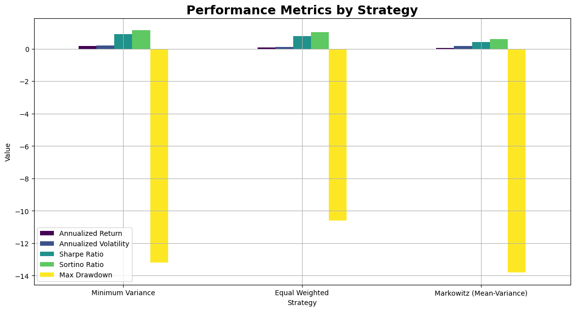
print(performance_df)
                           Annualized Return  Annualized Volatility  \
Minimum Variance                    0.186117               0.203196
Equal Weighted                      0.091404               0.116153
Markowitz (Mean-Variance)           0.071822               0.169583

                           Sharpe Ratio  Sortino Ratio  Max Drawdown
Minimum Variance               0.915950       1.149967    -13.204538
Equal Weighted                 0.786927       1.033226    -10.613445
Markowitz (Mean-Variance)      0.423524       0.605596    -13.811130
Plot performance metrics#
performance_df.plot(kind="bar", figsize=(14, 7), colormap="viridis")
plt.title("Performance Metrics by Strategy", fontsize=18, fontweight="bold")
plt.xlabel("Strategy")
plt.ylabel("Value")
plt.xticks(rotation=0)
plt.grid(True)
plt.show()