Pairs Trading Strategy Optimization in Python with AMPL#
![]()
![]()


![]()

Description: Optimize pairs trading strategy by optimizing entry and exit thresholds for each pair based on training data. This approach uses interpolation to find optimal parameters within the range tested.
Tags: finance, pairs-trading
Notebook author: Mukeshwaran Baskaran <mukesh96official@gmail.com>
Introduction#
This notebook helps you understand and improve a trading strategy called “pairs trading.” It uses historical stock data to find the best times to buy and sell pairs of stocks. The goal is to make money by identifying when the prices of these stocks move away from their usual relationship and then return to normal. The notebook tests different trading parameters to find the ones that work best. It then uses AMPL to optimise these parameters, making the trading strategy more effective.
# Install dependencies
%pip install amplpy yfinance matplotlib pandas numpy -q
# Google Colab & Kaggle integration
from amplpy import AMPL, ampl_notebook

ampl = ampl_notebook(
    modules=["knitro"],  # modules to install
    license_uuid="default",  # license to use
)  # instantiate AMPL object and register magics
# Import libraries
import yfinance as yf
import pandas as pd
import numpy as np
import matplotlib.pyplot as plt
import os
import time
import logging
import matplotlib.colors as mcolors

# Define a list of distinct colors
colors = list(mcolors.TABLEAU_COLORS)  # Using Tableau colors for distinctiveness
# Define stock pairs and fetch data
STOCK_PAIRS = [
    ("AAPL", "MSFT"),  # Apple & Microsoft
    ("GOOGL", "META"),  # Google & Meta
    ("XOM", "CVX"),  # Exxon Mobil & Chevron
    ("AMZN", "WMT"),  # Amazon & Walmart
    ("PG", "UL"),  # Procter & Gamble & Unilever
    ("KO", "PEP"),  # Coca-Cola & PepsiCo
    ("INTC", "AMD"),  # Intel & Advanced Micro Devices
    ("TSLA", "NIO"),  # Tesla & NIO
    ("BMY", "LLY"),  # Bristol-Myers Squibb & Eli Lilly
    ("V", "MA"),  # Visa & Mastercard
]

START_DATE = "2015-01-01"
END_DATE = "2025-01-01"

# Configure logging
logging.basicConfig(
    level=logging.INFO, format="%(asctime)s - %(levelname)s - %(message)s"
)
Implementation#
Download historical data for stock pairs#
def fetch_stock_data(pairs, start_date, end_date, retries=3):
    """Fetch historical data for given stock pairs with retry mechanism."""
    data = {}
    for pair in pairs:
        ticker1, ticker2 = pair
        attempt = 0
        while attempt < retries:
            try:
                data[pair] = yf.download(
                    [ticker1, ticker2], start=start_date, end=end_date
                )["Close"]
                logging.info(f"Successfully fetched data for {ticker1}, {ticker2}")
                break  # Successfully fetched data, break out of retry loop
            except Exception as e:
                logging.error(f"Error fetching data for {ticker1}, {ticker2}: {e}")
                attempt += 1
                if attempt < retries:
                    logging.info(f"Retrying... ({attempt}/{retries})")
                    time.sleep(5)  # Wait before retrying
                else:
                    logging.error(
                        f"Failed to fetch data after {retries} attempts for {ticker1}, {ticker2}"
                    )
    return data
Calculate spread and z-score#
def calculate_spread_zscore(data, lookback=30):
    """Calculate spread and z-score for each pair."""
    spreads = {}
    z_scores = {}
    for pair in data:
        ticker1, ticker2 = pair
        spread = data[pair][ticker1] - data[pair][ticker2]
        spread_mean = spread.rolling(window=lookback).mean()
        spread_std = spread.rolling(window=lookback).std()
        z_score = (spread - spread_mean) / spread_std
        spreads[pair] = spread
        z_scores[pair] = z_score
    return spreads, z_scores
Backtest pairs trading strategy with pair-specific parameters#
def backtest_pairs_trading(data, z_scores, pair_params):
    """
    Backtest a pairs trading strategy using pair-specific parameters.

    Args:
        data: Dictionary of price data
        z_scores: Dictionary of z-scores
        pair_params: Dictionary mapping pair strings to (entry_threshold, exit_threshold) tuples
    """
    results = {}
    for pair in data:
        ticker1, ticker2 = pair
        pair_key = f"{ticker1}_{ticker2}"

        # Get pair-specific parameters or use defaults
        entry_threshold, exit_threshold = pair_params.get(pair_key, (1.0, 0.5))

        z_score = z_scores[pair]
        positions = pd.Series(0, index=z_score.index)
        returns = pd.Series(0.0, index=z_score.index)

        # Generate trading signals
        long_entry = z_score < -entry_threshold
        short_entry = z_score > entry_threshold
        long_exit = z_score > -exit_threshold
        short_exit = z_score < exit_threshold

        # Simulate trades
        position = 0
        for i in range(1, len(z_score)):
            if long_entry.iloc[i] and position <= 0:
                position = 1  # Go long
            elif short_entry.iloc[i] and position >= 0:
                position = -1  # Go short
            elif (long_exit.iloc[i] and position == 1) or (
                short_exit.iloc[i] and position == -1
            ):
                position = 0  # Exit position

            positions.iloc[i] = position
            returns.iloc[i] = (
                position
                * (data[pair][ticker1].iloc[i] - data[pair][ticker1].iloc[i - 1])
                / data[pair][ticker1].iloc[i - 1]
            )

        # Calculate drawdown
        cumulative_returns = returns.cumsum()
        drawdown = cumulative_returns - cumulative_returns.cummax()

        # Store results
        results[pair_key] = {
            "positions": positions,
            "returns": returns,
            "cumulative_returns": cumulative_returns,
            "drawdown": drawdown,
            "sharpe_ratio": (
                (returns.mean() / returns.std()) * np.sqrt(252)
                if returns.std() > 0
                else 0
            ),
        }
    return results
Create training data for AMPL optimization#
def create_training_data(stock_data, z_scores, pairs, num_samples=20):
    """
    Generate training data for AMPL by running backtests with different parameters.

    Args:
        stock_data: Dictionary of price data
        z_scores: Dictionary of z-scores
        pairs: List of stock pairs
        num_samples: Number of parameter combinations to test

    Returns:
        Dictionary with pairs as keys and lists of (entry, exit, sharpe) tuples as values
    """
    # Define parameter ranges
    entry_range = np.linspace(0.5, 2.5, int(np.sqrt(num_samples)))
    exit_range = np.linspace(0.1, 1.5, int(np.sqrt(num_samples)))

    training_data = {}

    for pair in pairs:
        ticker1, ticker2 = pair
        pair_key = f"{ticker1}_{ticker2}"
        training_data[pair_key] = []

        logging.info(f"Generating training data for {pair_key}...")

        # Generate parameter combinations where entry >= exit
        valid_combinations = [(e, x) for e in entry_range for x in exit_range if e >= x]

        for entry, exit in valid_combinations:
            # Test this parameter combination
            test_params = {pair_key: (entry, exit)}
            results = backtest_pairs_trading(
                {pair: stock_data[pair]}, {pair: z_scores[pair]}, test_params
            )
            sharpe = results[pair_key]["sharpe_ratio"]

            # Store the parameter combination and resulting Sharpe ratio
            training_data[pair_key].append((entry, exit, sharpe))

    return training_data
Optimize parameters for each pair independently#
def optimize_pair_parameters(stock_data, z_scores):
    """
    Optimize parameters for each pair individually using grid search approach.
    Returns a dictionary with optimal parameters for each pair.
    """
    # Define search grid - can be adjusted for finer/broader search
    entry_thresholds = np.linspace(0.5, 2.5, 5)  # [0.5, 1.0, 1.5, 2.0, 2.5]
    exit_thresholds = np.linspace(0.1, 1.5, 5)  # [0.1, 0.4, 0.7, 1.0, 1.3]

    optimal_params = {}

    for pair in stock_data:
        ticker1, ticker2 = pair
        pair_key = f"{ticker1}_{ticker2}"

        best_sharpe = -np.inf
        best_params = (1.0, 0.5)  # Default

        logging.info(f"Optimizing parameters for pair: {pair_key}")

        for entry in entry_thresholds:
            for exit in exit_thresholds:
                # Skip invalid combinations (entry must be >= exit)
                if entry < exit:
                    continue

                # Test this parameter combination
                test_params = {pair_key: (entry, exit)}
                results = backtest_pairs_trading(
                    {pair: stock_data[pair]}, {pair: z_scores[pair]}, test_params
                )
                sharpe = results[pair_key]["sharpe_ratio"]

                if sharpe > best_sharpe:
                    best_sharpe = sharpe
                    best_params = (entry, exit)

        logging.info(
            f"Optimal parameters for {pair_key}: Entry={best_params[0]:.2f}, Exit={best_params[1]:.2f}, Sharpe={best_sharpe:.4f}"
        )
        optimal_params[pair_key] = best_params

    return optimal_params
Optimize parameters using AMPL for each pair#
def optimize_with_ampl(training_data):
    """
    Use AMPL to optimize entry and exit thresholds for each pair based on training data.

    This approach uses interpolation to find optimal parameters within the range tested.
    """
    optimal_params = {}

    for pair_key in training_data:
        logging.info(f"Optimizing parameters for {pair_key} using AMPL...")

        # Extract training data for this pair
        pair_data = training_data[pair_key]
        entry_values = [p[0] for p in pair_data]
        exit_values = [p[1] for p in pair_data]
        sharpe_values = [p[2] for p in pair_data]

        ampl = AMPL()

        # Define AMPL model for interpolation and optimization
        ampl.eval(
            r"""
            # Sets for parameter combinations
            set SAMPLES;

            # Parameters for each sample
            param entry_threshold {SAMPLES};
            param exit_threshold {SAMPLES};
            param sharpe_ratio {SAMPLES};

            # Decision variables for optimal thresholds
            var opt_entry >= 0.5, <= 2.5;
            var opt_exit >= 0.1, <= 1.5;

            # RBF kernel function for interpolation (Gaussian)
            param sigma := 0.3;  # Width parameter for RBF kernel

            # RBF kernel function: exp(-||x - y||^2 / (2*sigma^2))
            var rbf_kernel{s in SAMPLES} = exp(-((opt_entry - entry_threshold[s])^2 + (opt_exit - exit_threshold[s])^2) / (2*sigma^2));

            # Interpolated objective function using RBF kernel
            maximize predicted_sharpe:
                sum {s in SAMPLES} sharpe_ratio[s] * rbf_kernel[s] /
                sum {t in SAMPLES} rbf_kernel[t];

            # Constraint: entry threshold must be greater than or equal to exit threshold
            subject to threshold_constraint:
                opt_entry >= opt_exit;
        """
        )

        # Set data in AMPL
        ampl.set["SAMPLES"] = list(range(len(pair_data)))
        ampl.param["entry_threshold"] = {
            i: pair_data[i][0] for i in range(len(pair_data))
        }
        ampl.param["exit_threshold"] = {
            i: pair_data[i][1] for i in range(len(pair_data))
        }
        ampl.param["sharpe_ratio"] = {i: pair_data[i][2] for i in range(len(pair_data))}

        # Solve the optimization problem
        try:
            ampl.solve(solver="knitro", knitro_options="outlev=1")
            assert ampl.solve_result == "solved", ampl.solve_result

            # Extract optimized parameters
            opt_entry = ampl.var["opt_entry"].value()
            opt_exit = ampl.var["opt_exit"].value()
            predicted_sharpe = ampl.obj["predicted_sharpe"].value()

            logging.info(
                f"AMPL optimization for {pair_key}: Entry={opt_entry:.2f}, Exit={opt_exit:.2f}, Predicted Sharpe={predicted_sharpe:.4f}"
            )

            optimal_params[pair_key] = (opt_entry, opt_exit)
        except Exception as e:
            logging.error(f"AMPL optimization failed for {pair_key}: {e}")
            # Fallback to best sample if optimization fails
            best_idx = np.argmax(sharpe_values)
            optimal_params[pair_key] = (entry_values[best_idx], exit_values[best_idx])
            logging.info(
                f"Falling back to best sample: Entry={entry_values[best_idx]:.2f}, Exit={exit_values[best_idx]:.2f}"
            )

    return optimal_params
Plot parameter heatmap with AMPL solution#
def plot_parameter_heatmap(training_data, optimal_params, pair_key):
    """Plot heatmap of Sharpe ratios with AMPL's optimal solution."""
    # Extract data for visualization
    entry_values = [p[0] for p in training_data[pair_key]]
    exit_values = [p[1] for p in training_data[pair_key]]
    sharpe_values = [p[2] for p in training_data[pair_key]]

    # Create a grid for the heatmap
    entry_grid = np.linspace(min(entry_values), max(entry_values), 50)
    exit_grid = np.linspace(min(exit_values), max(exit_values), 50)

    # Create mesh grid
    X, Y = np.meshgrid(exit_grid, entry_grid)
    Z = np.zeros(X.shape)

    # Fill Z with interpolated values using RBF kernel
    sigma = 0.3  # Same as in AMPL model
    for i in range(Z.shape[0]):
        for j in range(Z.shape[1]):
            if entry_grid[i] < exit_grid[j]:  # Skip invalid regions
                Z[i, j] = np.nan
                continue

            # RBF interpolation
            weights = np.exp(
                -(
                    (entry_grid[i] - np.array(entry_values)) ** 2
                    + (exit_grid[j] - np.array(exit_values)) ** 2
                )
                / (2 * sigma**2)
            )
            if np.sum(weights) > 0:
                Z[i, j] = np.sum(weights * np.array(sharpe_values)) / np.sum(weights)
            else:
                Z[i, j] = np.nan

    # Create plot
    plt.figure(figsize=(10, 8))

    # Plot heatmap
    cmap = plt.cm.viridis
    cmap.set_bad("white", 1.0)
    heatmap = plt.pcolormesh(X, Y, Z, cmap=cmap, shading="auto")

    plt.colorbar(heatmap, label="Interpolated Sharpe Ratio")
    plt.title(f"Parameter Optimization Landscape for {pair_key}")
    plt.xlabel("Exit Threshold")
    plt.ylabel("Entry Threshold")

    # Add contour lines
    contour = plt.contour(X, Y, Z, colors="white", alpha=0.5)
    plt.clabel(contour, inline=True, fontsize=8)

    # Plot training data points
    plt.scatter(
        exit_values,
        entry_values,
        c=sharpe_values,
        cmap="viridis",
        s=50,
        edgecolor="black",
        label="Training Samples",
    )

    # Mark the AMPL optimal solution
    opt_entry, opt_exit = optimal_params[pair_key]
    plt.scatter(
        [opt_exit],
        [opt_entry],
        color="red",
        s=200,
        marker="*",
        label=f"AMPL Optimal: Entry={opt_entry:.2f}, Exit={opt_exit:.2f}",
    )

    # Diagonal line showing the constraint boundary
    diag_x = np.linspace(min(exit_grid), max(exit_grid), 100)
    plt.plot(diag_x, diag_x, "r--", alpha=0.7, label="Constraint: Entry ≥ Exit")

    plt.legend()
    plt.tight_layout()
    plt.show()
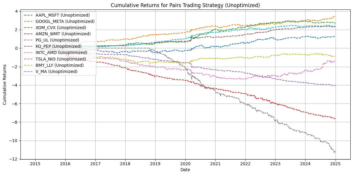
Plot cumulative returns for unoptimized strategy#
def plot_cumulative_returns_unoptimized(unoptimized_results):
    """Plot cumulative returns for unoptimized strategy."""
    plt.figure(figsize=(12, 6))

    # Plot unoptimized cumulative returns with different colors
    for i, pair in enumerate(unoptimized_results):
        plt.plot(
            unoptimized_results[pair]["cumulative_returns"],
            label=f"{pair} (Unoptimized)",
            linestyle="--",
            color=colors[i % len(colors)],
        )

    plt.title("Cumulative Returns for Pairs Trading Strategy (Unoptimized)")
    plt.xlabel("Date")
    plt.ylabel("Cumulative Returns")
    plt.legend(loc="upper left")
    plt.grid(True)
    plt.tight_layout()
    plt.show()
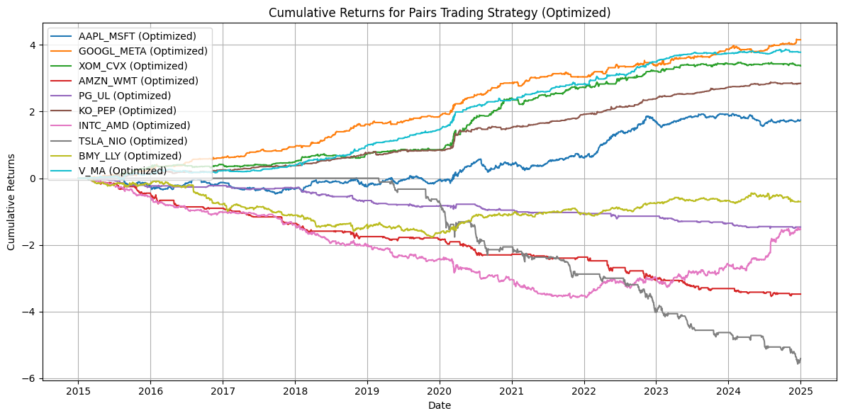
Plot cumulative returns for optimized strategy#
def plot_cumulative_returns_optimized(optimized_results):
    """Plot cumulative returns for optimized strategy."""
    plt.figure(figsize=(12, 6))

    # Plot optimized cumulative returns with different colors
    for i, pair in enumerate(optimized_results):
        plt.plot(
            optimized_results[pair]["cumulative_returns"],
            label=f"{pair} (Optimized)",
            linestyle="-",
            color=colors[i % len(colors)],
        )

    plt.title("Cumulative Returns for Pairs Trading Strategy (Optimized)")
    plt.xlabel("Date")
    plt.ylabel("Cumulative Returns")
    plt.legend(loc="upper left")
    plt.grid(True)
    plt.tight_layout()
    plt.show()
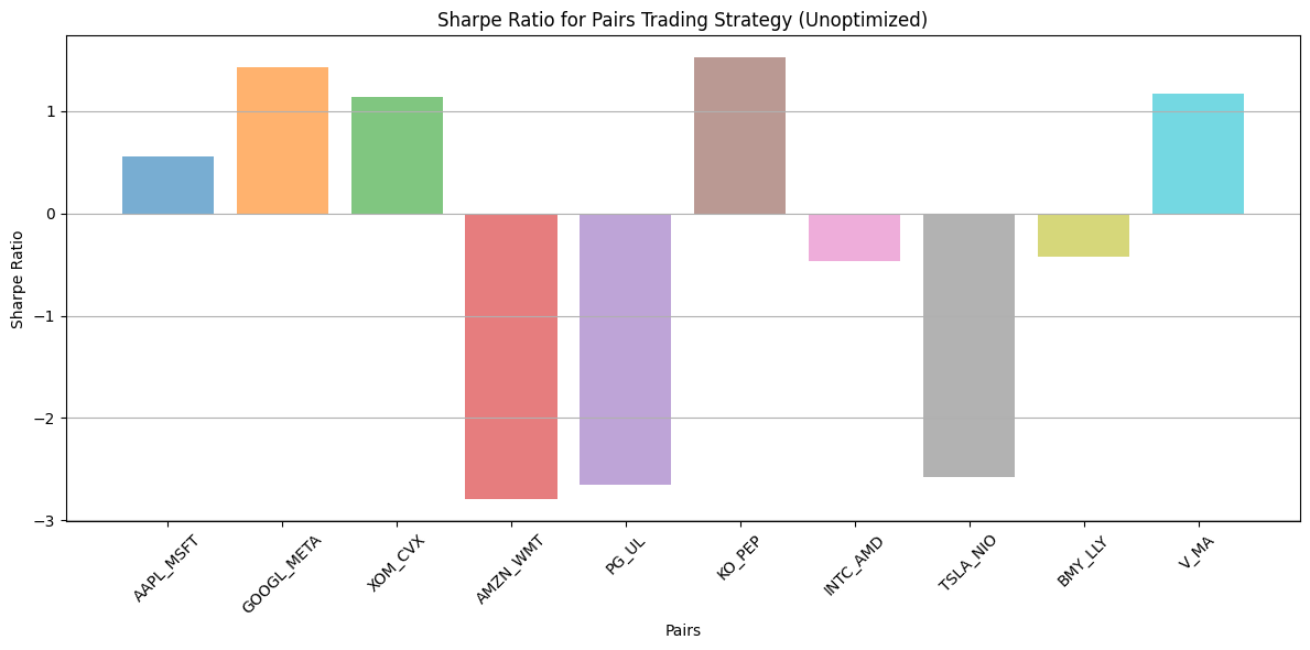
Plot Sharpe ratio for unoptimized strategy#
def plot_sharpe_ratio_unoptimized(unoptimized_results):
    """Plot Sharpe ratio for unoptimized strategy."""
    sharpe_ratios_before = {
        pair: unoptimized_results[pair]["sharpe_ratio"] for pair in unoptimized_results
    }

    plt.figure(figsize=(12, 6))

    # Plot Sharpe ratios for unoptimized with different colors
    for i, pair in enumerate(sharpe_ratios_before):
        plt.bar(
            i,
            sharpe_ratios_before[pair],
            label=f"{pair}",
            alpha=0.6,
            color=colors[i % len(colors)],
        )

    plt.title("Sharpe Ratio for Pairs Trading Strategy (Unoptimized)")
    plt.xlabel("Pairs")
    plt.ylabel("Sharpe Ratio")
    plt.xticks(
        range(len(sharpe_ratios_before)), sharpe_ratios_before.keys(), rotation=45
    )
    plt.tight_layout()
    plt.grid(True, axis="y")
    plt.show()
Plot Sharpe ratio for optimized strategy#
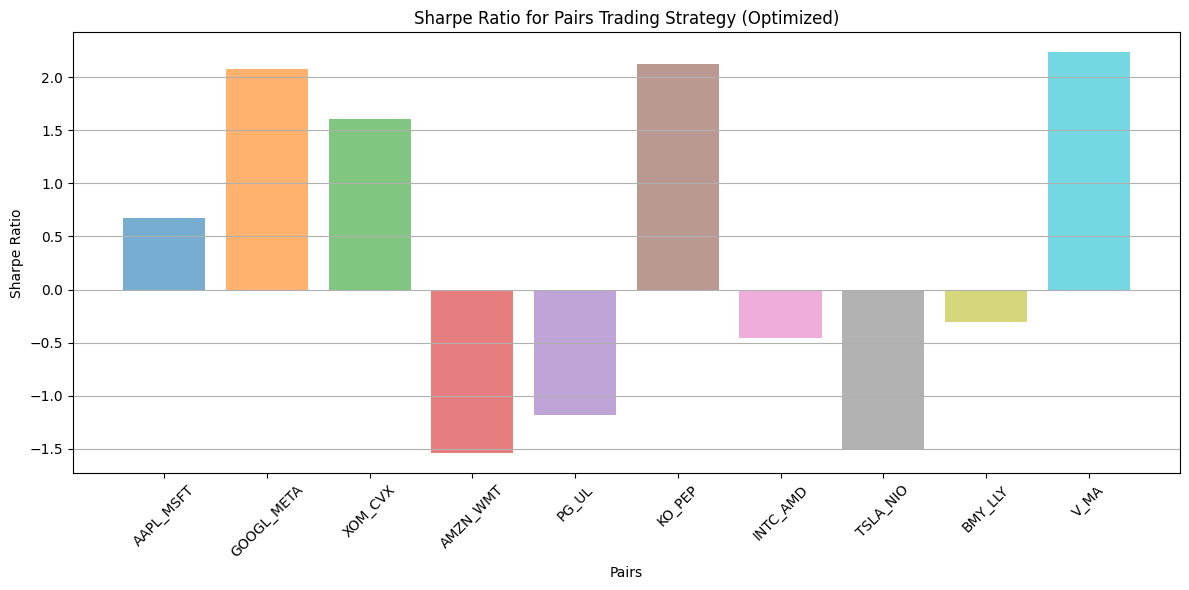
def plot_sharpe_ratio_optimized(optimized_results):
    """Plot Sharpe ratio for optimized strategy."""
    sharpe_ratios_after = {
        pair: optimized_results[pair]["sharpe_ratio"] for pair in optimized_results
    }

    plt.figure(figsize=(12, 6))

    # Plot Sharpe ratios for optimized with different colors
    for i, pair in enumerate(sharpe_ratios_after):
        plt.bar(
            i,
            sharpe_ratios_after[pair],
            label=f"{pair}",
            alpha=0.6,
            color=colors[i % len(colors)],
        )

    plt.title("Sharpe Ratio for Pairs Trading Strategy (Optimized)")
    plt.xlabel("Pairs")
    plt.ylabel("Sharpe Ratio")
    plt.xticks(range(len(sharpe_ratios_after)), sharpe_ratios_after.keys(), rotation=45)
    plt.tight_layout()
    plt.grid(True, axis="y")
    plt.show()
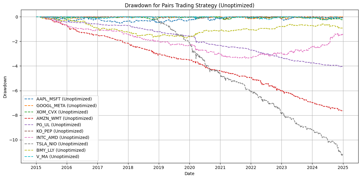
Plot drawdown for unoptimized strategy#
def plot_drawdown_unoptimized(unoptimized_results):
    """Plot drawdown for unoptimized strategy."""
    plt.figure(figsize=(12, 6))

    # Plot unoptimized drawdowns with different colors
    for i, pair in enumerate(unoptimized_results):
        plt.plot(
            unoptimized_results[pair]["drawdown"],
            label=f"{pair} (Unoptimized)",
            linestyle="--",
            color=colors[i % len(colors)],
        )

    plt.title("Drawdown for Pairs Trading Strategy (Unoptimized)")
    plt.xlabel("Date")
    plt.ylabel("Drawdown")
    plt.legend(loc="lower left")
    plt.grid(True)
    plt.tight_layout()
    plt.show()
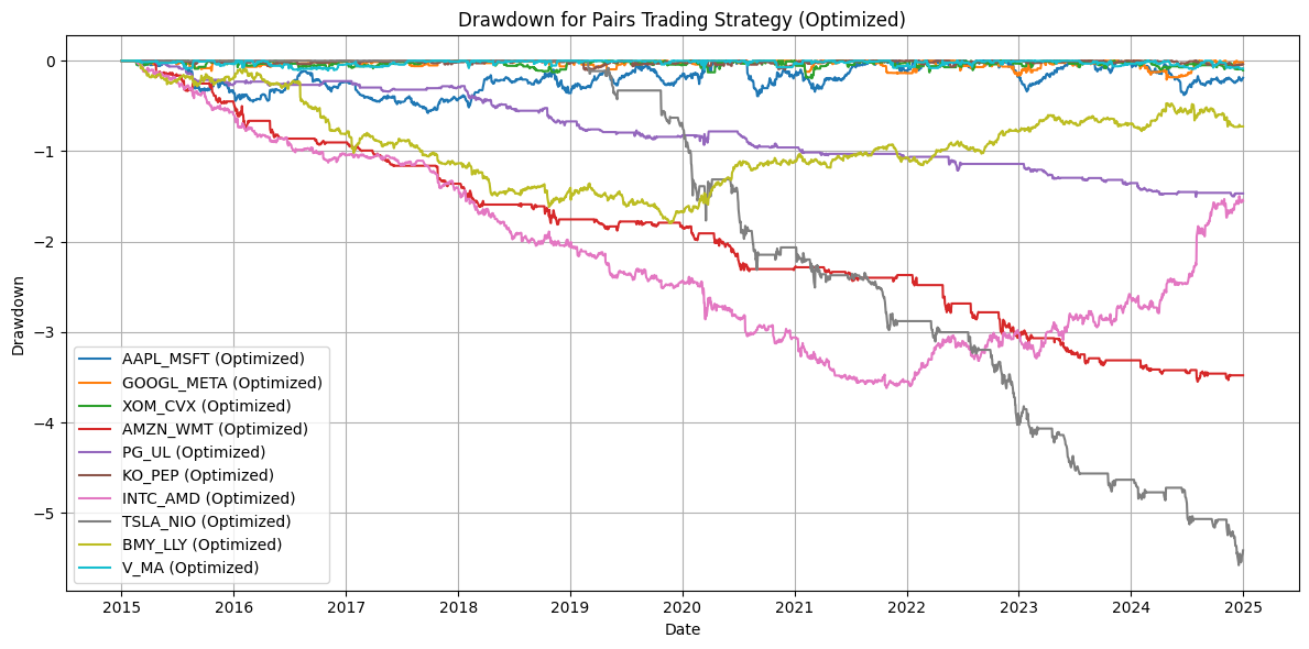
Plot drawdown for optimized strategy#
def plot_drawdown_optimized(optimized_results):
    """Plot drawdown for optimized strategy."""
    plt.figure(figsize=(12, 6))

    # Plot optimized drawdowns with different colors
    for i, pair in enumerate(optimized_results):
        plt.plot(
            optimized_results[pair]["drawdown"],
            label=f"{pair} (Optimized)",
            linestyle="-",
            color=colors[i % len(colors)],
        )

    plt.title("Drawdown for Pairs Trading Strategy (Optimized)")
    plt.xlabel("Date")
    plt.ylabel("Drawdown")
    plt.legend(loc="lower left")
    plt.grid(True)
    plt.tight_layout()
    plt.show()
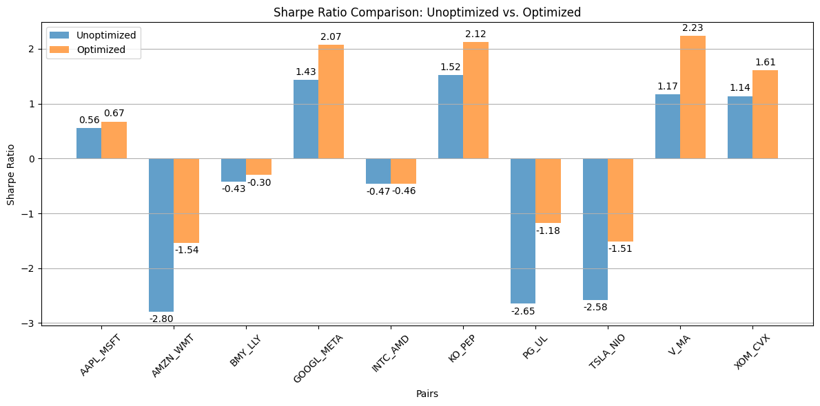
Plot comparison of unoptimized vs optimized Sharpe ratios#
def plot_sharpe_comparison(unoptimized_results, optimized_results):
    """Plot comparison of Sharpe ratios before and after optimization."""
    pairs = sorted(unoptimized_results.keys())
    sharpe_before = [unoptimized_results[p]["sharpe_ratio"] for p in pairs]
    sharpe_after = [optimized_results[p]["sharpe_ratio"] for p in pairs]

    x = np.arange(len(pairs))
    width = 0.35

    fig, ax = plt.subplots(figsize=(12, 6))
    rects1 = ax.bar(x - width / 2, sharpe_before, width, label="Unoptimized", alpha=0.7)
    rects2 = ax.bar(x + width / 2, sharpe_after, width, label="Optimized", alpha=0.7)

    ax.set_title("Sharpe Ratio Comparison: Unoptimized vs. Optimized")
    ax.set_xlabel("Pairs")
    ax.set_ylabel("Sharpe Ratio")
    ax.set_xticks(x)
    ax.set_xticklabels(pairs, rotation=45)
    ax.legend()

    ax.bar_label(rects1, padding=3, fmt="%.2f")
    ax.bar_label(rects2, padding=3, fmt="%.2f")

    fig.tight_layout()
    plt.grid(True, axis="y")
    plt.show()
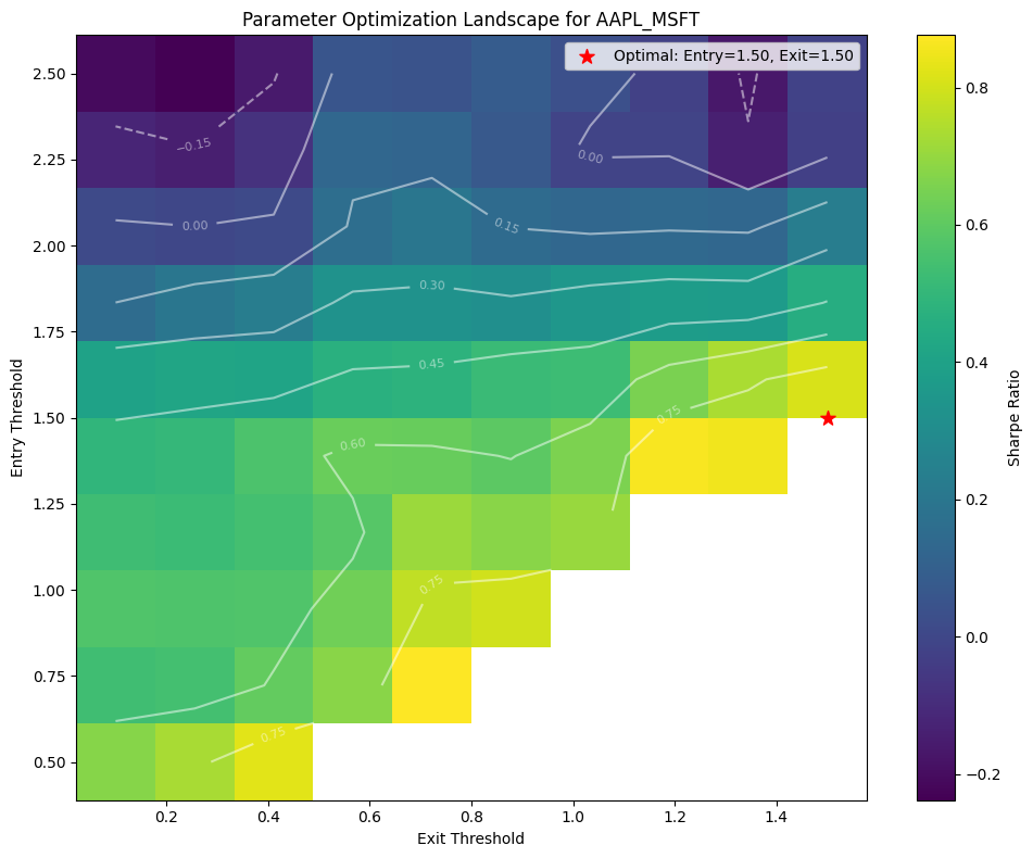
Plot parameter heatmap to visualize the optimization landscape for a specific pair#
def plot_parameter_heatmap(stock_data, z_scores, pair_index=0):
    """Plot heatmap of Sharpe ratios for different parameter combinations."""
    # Select a pair for visualization
    pair = list(stock_data.keys())[pair_index]
    ticker1, ticker2 = pair
    pair_key = f"{ticker1}_{ticker2}"

    # Define search grid with finer resolution for visualization
    entry_thresholds = np.linspace(0.5, 2.5, 10)
    exit_thresholds = np.linspace(0.1, 1.5, 10)

    # Create empty grid for heatmap data
    sharpe_grid = np.zeros((len(entry_thresholds), len(exit_thresholds)))
    sharpe_grid[:] = np.nan  # Fill with NaN for invalid combinations

    # Calculate Sharpe ratios for parameter combinations
    for i, entry in enumerate(entry_thresholds):
        for j, exit in enumerate(exit_thresholds):
            # Skip invalid combinations (entry must be >= exit)
            if entry < exit:
                continue

            # Test this parameter combination
            test_params = {pair_key: (entry, exit)}
            results = backtest_pairs_trading(
                {pair: stock_data[pair]}, {pair: z_scores[pair]}, test_params
            )
            sharpe = results[pair_key]["sharpe_ratio"]
            sharpe_grid[i, j] = sharpe

    # Create heatmap
    plt.figure(figsize=(10, 8))
    heatmap = plt.pcolormesh(
        exit_thresholds, entry_thresholds, sharpe_grid, cmap="viridis", shading="auto"
    )

    plt.colorbar(heatmap, label="Sharpe Ratio")
    plt.title(f"Parameter Optimization Landscape for {pair_key}")
    plt.xlabel("Exit Threshold")
    plt.ylabel("Entry Threshold")

    # Add contour lines
    contour = plt.contour(
        exit_thresholds, entry_thresholds, sharpe_grid, colors="white", alpha=0.5
    )
    plt.clabel(contour, inline=True, fontsize=8)

    # Mark the optimal point
    optimal_params = optimize_pair_parameters(
        {pair: stock_data[pair]}, {pair: z_scores[pair]}
    )
    opt_entry, opt_exit = optimal_params[pair_key]
    plt.scatter(
        [opt_exit],
        [opt_entry],
        color="red",
        s=100,
        marker="*",
        label=f"Optimal: Entry={opt_entry:.2f}, Exit={opt_exit:.2f}",
    )

    plt.legend()
    plt.tight_layout()
    plt.show()
Print optimization summary showing parameters and performance#
def print_optimization_summary(
    optimized_params, unoptimized_results, optimized_results
):
    """Print a summary of the optimization results."""
    print("\n" + "=" * 80)
    print("PAIRS TRADING STRATEGY OPTIMIZATION SUMMARY")
    print("=" * 80)

    print("\nOptimized Parameters:")
    print("-" * 50)
    print(f"{'Pair':<15} {'Entry Threshold':<20} {'Exit Threshold':<20}")
    print("-" * 50)

    for pair_key in sorted(optimized_params.keys()):
        entry, exit = optimized_params[pair_key]
        print(f"{pair_key:<15} {entry:<20.2f} {exit:<20.2f}")

    print("\nPerformance Comparison:")
    print("-" * 80)
    print(
        f"{'Pair':<15} {'Unopt. Sharpe':<15} {'Opt. Sharpe':<15} {'Improvement':<15} {'% Change':<15}"
    )
    print("-" * 80)

    total_before = 0
    total_after = 0

    for pair_key in sorted(unoptimized_results.keys()):
        before = unoptimized_results[pair_key]["sharpe_ratio"]
        after = optimized_results[pair_key]["sharpe_ratio"]
        improvement = after - before
        percent_change = (
            (improvement / abs(before)) * 100 if before != 0 else float("inf")
        )

        print(
            f"{pair_key:<15} {before:<15.4f} {after:<15.4f} {improvement:<+15.4f} {percent_change:<+15.2f}%"
        )

        total_before += before
        total_after += after

    total_improvement = total_after - total_before
    total_percent = (
        (total_improvement / abs(total_before)) * 100
        if total_before != 0
        else float("inf")
    )

    print("-" * 80)
    print(
        f"{'TOTAL':<15} {total_before:<15.4f} {total_after:<15.4f} {total_improvement:<+15.4f} {total_percent:<+15.2f}%"
    )
    print("=" * 80)
Compare all metrics between optimized and unoptimized strategies#
def compare_strategies(unoptimized_results, optimized_results):
    """Calculate and compare key metrics between strategies."""
    metrics = {}

    for strategy, results in [
        ("Unoptimized", unoptimized_results),
        ("Optimized", optimized_results),
    ]:
        # Calculate portfolio-level metrics
        all_returns = pd.DataFrame({pair: results[pair]["returns"] for pair in results})
        portfolio_returns = all_returns.mean(axis=1)  # Equal-weighted portfolio

        cum_returns = portfolio_returns.cumsum()
        drawdown = cum_returns - cum_returns.cummax()

        # Calculate metrics
        metrics[strategy] = {
            "Total Return": cum_returns.iloc[-1],
            "Annualized Return": portfolio_returns.mean() * 252,
            "Annualized Volatility": portfolio_returns.std() * np.sqrt(252),
            "Sharpe Ratio": (portfolio_returns.mean() / portfolio_returns.std())
            * np.sqrt(252),
            "Max Drawdown": drawdown.min(),
            "Calmar Ratio": (
                (portfolio_returns.mean() * 252) / abs(drawdown.min())
                if drawdown.min() < 0
                else np.inf
            ),
            "Winning Pairs": sum(
                1 for p in results if results[p]["cumulative_returns"].iloc[-1] > 0
            ),
            "Total Pairs": len(results),
        }

    # Create comparison DataFrame
    comparison = pd.DataFrame({k: v for k, v in metrics.items()})

    # Calculate improvement
    improvement = comparison["Optimized"] - comparison["Unoptimized"]
    percent_change = (improvement / comparison["Unoptimized"].abs()) * 100

    comparison["Improvement"] = improvement
    comparison["% Change"] = percent_change

    return comparison
Plot portfolio returns comparison#
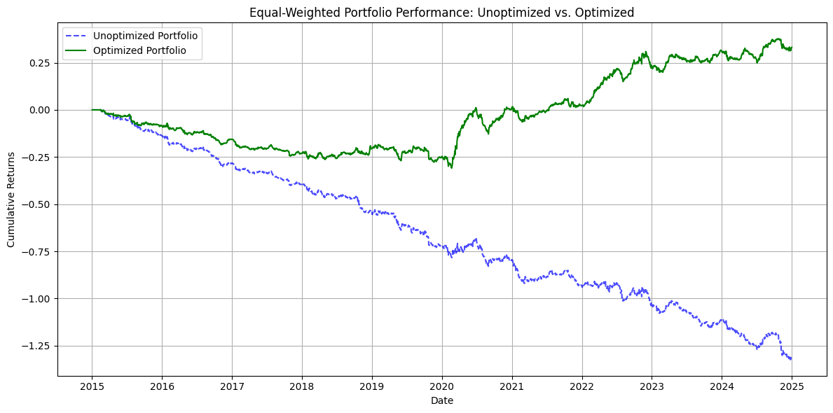
def plot_portfolio_comparison(unoptimized_results, optimized_results):
    """Plot comparison of portfolio returns."""
    # Calculate portfolio returns for each strategy
    unopt_returns = pd.DataFrame(
        {pair: unoptimized_results[pair]["returns"] for pair in unoptimized_results}
    )
    opt_returns = pd.DataFrame(
        {pair: optimized_results[pair]["returns"] for pair in optimized_results}
    )

    unopt_portfolio = unopt_returns.mean(axis=1).cumsum()
    opt_portfolio = opt_returns.mean(axis=1).cumsum()

    # Plot comparison
    plt.figure(figsize=(12, 6))
    plt.plot(
        unopt_portfolio,
        label="Unoptimized Portfolio",
        linestyle="--",
        color="blue",
        alpha=0.7,
    )
    plt.plot(opt_portfolio, label="Optimized Portfolio", linestyle="-", color="green")

    plt.title("Equal-Weighted Portfolio Performance: Unoptimized vs. Optimized")
    plt.xlabel("Date")
    plt.ylabel("Cumulative Returns")
    plt.legend()
    plt.grid(True)
    plt.tight_layout()
    plt.show()
Execution#
Fetch data#
logging.info("Fetching stock data...")
stock_data = fetch_stock_data(STOCK_PAIRS, START_DATE, END_DATE)
[*********************100%***********************]  2 of 2 completed
[*********************100%***********************]  2 of 2 completed
[*********************100%***********************]  2 of 2 completed
[*********************100%***********************]  2 of 2 completed
[*********************100%***********************]  2 of 2 completed
[*********************100%***********************]  2 of 2 completed
[*********************100%***********************]  2 of 2 completed
[*********************100%***********************]  2 of 2 completed
[*********************100%***********************]  2 of 2 completed
[*********************100%***********************]  2 of 2 completed
Calculate spread and z-score#
logging.info("Calculating spreads and z-scores...")
spreads, z_scores = calculate_spread_zscore(stock_data)
Default parameters for unoptimized strategy#
default_entry_threshold = 1.0
default_exit_threshold = 0.5
default_params = {
    f"{p[0]}_{p[1]}": (default_entry_threshold, default_exit_threshold)
    for p in stock_data
}
Backtest with default parameters#
logging.info("Running backtest with default parameters...")
unoptimized_results = backtest_pairs_trading(stock_data, z_scores, default_params)
Optimize parameters for each pair#
logging.info("Starting parameter optimization for each pair...")
# optimized_params = optimize_pair_parameters(stock_data, z_scores)
training_data = create_training_data(stock_data, z_scores, STOCK_PAIRS, num_samples=20)
optimized_params = optimize_with_ampl(training_data)
Artelys Knitro 14.2.0: outlev=1
=======================================
Commercial License
Artelys Knitro 14.2.0
=======================================
Knitro presolve eliminated 0 variables and 0 constraints.
concurrent_evals 0
datacheck 0
findiff_numthreads 1
hessian_no_f 1
hessopt 1
outlev 1
The problem is linearly constrained.
Problem Characteristics ( Presolved)
-----------------------
Objective goal: Maximize
Objective type: general
Number of variables: 2 ( 2)
bounded below only: 0 ( 0)
bounded above only: 0 ( 0)
bounded below and above: 2 ( 2)
fixed: 0 ( 0)
free: 0 ( 0)
Number of constraints: 1 ( 1)
linear equalities: 0 ( 0)
quadratic equalities: 0 ( 0)
gen. nonlinear equalities: 0 ( 0)
linear one-sided inequalities: 1 ( 1)
quadratic one-sided inequalities: 0 ( 0)
gen. nonlinear one-sided inequalities: 0 ( 0)
linear two-sided inequalities: 0 ( 0)
quadratic two-sided inequalities: 0 ( 0)
gen. nonlinear two-sided inequalities: 0 ( 0)
Number of nonzeros in Jacobian: 2 ( 2)
Number of nonzeros in Hessian: 3 ( 3)
Knitro using the Interior-Point/Barrier Direct algorithm.
EXIT: Locally optimal solution found.
Final Statistics
----------------
Final objective value = 6.60226460566116e-01
Final feasibility error (abs / rel) = 0.00e+00 / 0.00e+00
Final optimality error (abs / rel) = 1.12e-12 / 1.12e-12
# of iterations = 6
# of CG iterations = 2
# of function evaluations = 8
# of gradient evaluations = 8
# of Hessian evaluations = 6
Total program time (secs) = 0.01247 ( 0.002 CPU time)
Time spent in evaluations (secs) = 0.00013
===============================================================================
Knitro 14.2.0: Locally optimal or satisfactory solution.
objective 0.6602264606; feasibility error 0
6 iterations; 8 function evaluations
suffix feaserror OUT;
suffix opterror OUT;
suffix numfcevals OUT;
suffix numiters OUT;
Artelys Knitro 14.2.0: outlev=1
=======================================
Commercial License
Artelys Knitro 14.2.0
=======================================
Knitro presolve eliminated 0 variables and 0 constraints.
concurrent_evals 0
datacheck 0
findiff_numthreads 1
hessian_no_f 1
hessopt 1
outlev 1
The problem is linearly constrained.
Problem Characteristics ( Presolved)
-----------------------
Objective goal: Maximize
Objective type: general
Number of variables: 2 ( 2)
bounded below only: 0 ( 0)
bounded above only: 0 ( 0)
bounded below and above: 2 ( 2)
fixed: 0 ( 0)
free: 0 ( 0)
Number of constraints: 1 ( 1)
linear equalities: 0 ( 0)
quadratic equalities: 0 ( 0)
gen. nonlinear equalities: 0 ( 0)
linear one-sided inequalities: 1 ( 1)
quadratic one-sided inequalities: 0 ( 0)
gen. nonlinear one-sided inequalities: 0 ( 0)
linear two-sided inequalities: 0 ( 0)
quadratic two-sided inequalities: 0 ( 0)
gen. nonlinear two-sided inequalities: 0 ( 0)
Number of nonzeros in Jacobian: 2 ( 2)
Number of nonzeros in Hessian: 3 ( 3)
Knitro using the Interior-Point/Barrier Direct algorithm.
EXIT: Locally optimal solution found.
Final Statistics
----------------
Final objective value = 1.72882455097880e+00
Final feasibility error (abs / rel) = 0.00e+00 / 0.00e+00
Final optimality error (abs / rel) = 4.27e-10 / 4.27e-10
# of iterations = 5
# of CG iterations = 1
# of function evaluations = 7
# of gradient evaluations = 7
# of Hessian evaluations = 5
Total program time (secs) = 0.01283 ( 0.002 CPU time)
Time spent in evaluations (secs) = 0.00009
===============================================================================
Knitro 14.2.0: Locally optimal or satisfactory solution.
objective 1.728824551; feasibility error 0
5 iterations; 7 function evaluations
suffix feaserror OUT;
suffix opterror OUT;
suffix numfcevals OUT;
suffix numiters OUT;
Artelys Knitro 14.2.0: outlev=1
=======================================
Commercial License
Artelys Knitro 14.2.0
=======================================
Knitro presolve eliminated 0 variables and 0 constraints.
concurrent_evals 0
datacheck 0
findiff_numthreads 1
hessian_no_f 1
hessopt 1
outlev 1
The problem is linearly constrained.
Problem Characteristics ( Presolved)
-----------------------
Objective goal: Maximize
Objective type: general
Number of variables: 2 ( 2)
bounded below only: 0 ( 0)
bounded above only: 0 ( 0)
bounded below and above: 2 ( 2)
fixed: 0 ( 0)
free: 0 ( 0)
Number of constraints: 1 ( 1)
linear equalities: 0 ( 0)
quadratic equalities: 0 ( 0)
gen. nonlinear equalities: 0 ( 0)
linear one-sided inequalities: 1 ( 1)
quadratic one-sided inequalities: 0 ( 0)
gen. nonlinear one-sided inequalities: 0 ( 0)
linear two-sided inequalities: 0 ( 0)
quadratic two-sided inequalities: 0 ( 0)
gen. nonlinear two-sided inequalities: 0 ( 0)
Number of nonzeros in Jacobian: 2 ( 2)
Number of nonzeros in Hessian: 3 ( 3)
Knitro using the Interior-Point/Barrier Direct algorithm.
EXIT: Locally optimal solution found.
Final Statistics
----------------
Final objective value = 1.22894685859887e+00
Final feasibility error (abs / rel) = 0.00e+00 / 0.00e+00
Final optimality error (abs / rel) = 1.83e-07 / 1.83e-07
# of iterations = 5
# of CG iterations = 1
# of function evaluations = 7
# of gradient evaluations = 7
# of Hessian evaluations = 5
Total program time (secs) = 0.01388 ( 0.002 CPU time)
Time spent in evaluations (secs) = 0.00007
===============================================================================
Knitro 14.2.0: Locally optimal or satisfactory solution.
objective 1.228946859; feasibility error 0
5 iterations; 7 function evaluations
suffix feaserror OUT;
suffix opterror OUT;
suffix numfcevals OUT;
suffix numiters OUT;
Artelys Knitro 14.2.0: outlev=1
=======================================
Commercial License
Artelys Knitro 14.2.0
=======================================
Knitro presolve eliminated 0 variables and 0 constraints.
concurrent_evals 0
datacheck 0
findiff_numthreads 1
hessian_no_f 1
hessopt 1
outlev 1
The problem is linearly constrained.
Problem Characteristics ( Presolved)
-----------------------
Objective goal: Maximize
Objective type: general
Number of variables: 2 ( 2)
bounded below only: 0 ( 0)
bounded above only: 0 ( 0)
bounded below and above: 2 ( 2)
fixed: 0 ( 0)
free: 0 ( 0)
Number of constraints: 1 ( 1)
linear equalities: 0 ( 0)
quadratic equalities: 0 ( 0)
gen. nonlinear equalities: 0 ( 0)
linear one-sided inequalities: 1 ( 1)
quadratic one-sided inequalities: 0 ( 0)
gen. nonlinear one-sided inequalities: 0 ( 0)
linear two-sided inequalities: 0 ( 0)
quadratic two-sided inequalities: 0 ( 0)
gen. nonlinear two-sided inequalities: 0 ( 0)
Number of nonzeros in Jacobian: 2 ( 2)
Number of nonzeros in Hessian: 3 ( 3)
Knitro using the Interior-Point/Barrier Direct algorithm.
EXIT: Locally optimal solution found.
Final Statistics
----------------
Final objective value = -1.58414965720312e+00
Final feasibility error (abs / rel) = 0.00e+00 / 0.00e+00
Final optimality error (abs / rel) = 1.11e-08 / 1.11e-08
# of iterations = 5
# of CG iterations = 1
# of function evaluations = 7
# of gradient evaluations = 7
# of Hessian evaluations = 5
Total program time (secs) = 0.01037 ( 0.001 CPU time)
Time spent in evaluations (secs) = 0.00007
===============================================================================
Knitro 14.2.0: Locally optimal or satisfactory solution.
objective -1.584149657; feasibility error 0
5 iterations; 7 function evaluations
suffix feaserror OUT;
suffix opterror OUT;
suffix numfcevals OUT;
suffix numiters OUT;
Artelys Knitro 14.2.0: outlev=1
=======================================
Commercial License
Artelys Knitro 14.2.0
=======================================
Knitro presolve eliminated 0 variables and 0 constraints.
concurrent_evals 0
datacheck 0
findiff_numthreads 1
hessian_no_f 1
hessopt 1
outlev 1
The problem is linearly constrained.
Problem Characteristics ( Presolved)
-----------------------
Objective goal: Maximize
Objective type: general
Number of variables: 2 ( 2)
bounded below only: 0 ( 0)
bounded above only: 0 ( 0)
bounded below and above: 2 ( 2)
fixed: 0 ( 0)
free: 0 ( 0)
Number of constraints: 1 ( 1)
linear equalities: 0 ( 0)
quadratic equalities: 0 ( 0)
gen. nonlinear equalities: 0 ( 0)
linear one-sided inequalities: 1 ( 1)
quadratic one-sided inequalities: 0 ( 0)
gen. nonlinear one-sided inequalities: 0 ( 0)
linear two-sided inequalities: 0 ( 0)
quadratic two-sided inequalities: 0 ( 0)
gen. nonlinear two-sided inequalities: 0 ( 0)
Number of nonzeros in Jacobian: 2 ( 2)
Number of nonzeros in Hessian: 3 ( 3)
Knitro using the Interior-Point/Barrier Direct algorithm.
EXIT: Locally optimal solution found.
Final Statistics
----------------
Final objective value = -1.27901930071936e+00
Final feasibility error (abs / rel) = 0.00e+00 / 0.00e+00
Final optimality error (abs / rel) = 8.34e-11 / 8.34e-11
# of iterations = 6
# of CG iterations = 1
# of function evaluations = 8
# of gradient evaluations = 8
# of Hessian evaluations = 6
Total program time (secs) = 0.00437 ( 0.002 CPU time)
Time spent in evaluations (secs) = 0.00008
===============================================================================
Knitro 14.2.0: Locally optimal or satisfactory solution.
objective -1.279019301; feasibility error 0
6 iterations; 8 function evaluations
suffix feaserror OUT;
suffix opterror OUT;
suffix numfcevals OUT;
suffix numiters OUT;
Artelys Knitro 14.2.0: outlev=1
=======================================
Commercial License
Artelys Knitro 14.2.0
=======================================
Knitro presolve eliminated 0 variables and 0 constraints.
concurrent_evals 0
datacheck 0
findiff_numthreads 1
hessian_no_f 1
hessopt 1
outlev 1
The problem is linearly constrained.
Problem Characteristics ( Presolved)
-----------------------
Objective goal: Maximize
Objective type: general
Number of variables: 2 ( 2)
bounded below only: 0 ( 0)
bounded above only: 0 ( 0)
bounded below and above: 2 ( 2)
fixed: 0 ( 0)
free: 0 ( 0)
Number of constraints: 1 ( 1)
linear equalities: 0 ( 0)
quadratic equalities: 0 ( 0)
gen. nonlinear equalities: 0 ( 0)
linear one-sided inequalities: 1 ( 1)
quadratic one-sided inequalities: 0 ( 0)
gen. nonlinear one-sided inequalities: 0 ( 0)
linear two-sided inequalities: 0 ( 0)
quadratic two-sided inequalities: 0 ( 0)
gen. nonlinear two-sided inequalities: 0 ( 0)
Number of nonzeros in Jacobian: 2 ( 2)
Number of nonzeros in Hessian: 3 ( 3)
Knitro using the Interior-Point/Barrier Direct algorithm.
EXIT: Locally optimal solution found.
Final Statistics
----------------
Final objective value = 1.88225833653188e+00
Final feasibility error (abs / rel) = 0.00e+00 / 0.00e+00
Final optimality error (abs / rel) = 7.80e-08 / 7.80e-08
# of iterations = 4
# of CG iterations = 0
# of function evaluations = 7
# of gradient evaluations = 6
# of Hessian evaluations = 4
Total program time (secs) = 0.00400 ( 0.001 CPU time)
Time spent in evaluations (secs) = 0.00007
===============================================================================
Knitro 14.2.0: Locally optimal or satisfactory solution.
objective 1.882258337; feasibility error 0
4 iterations; 7 function evaluations
suffix feaserror OUT;
suffix opterror OUT;
suffix numfcevals OUT;
suffix numiters OUT;
Artelys Knitro 14.2.0: outlev=1
=======================================
Commercial License
Artelys Knitro 14.2.0
=======================================
Knitro presolve eliminated 0 variables and 0 constraints.
concurrent_evals 0
datacheck 0
findiff_numthreads 1
hessian_no_f 1
hessopt 1
outlev 1
The problem is linearly constrained.
Problem Characteristics ( Presolved)
-----------------------
Objective goal: Maximize
Objective type: general
Number of variables: 2 ( 2)
bounded below only: 0 ( 0)
bounded above only: 0 ( 0)
bounded below and above: 2 ( 2)
fixed: 0 ( 0)
free: 0 ( 0)
Number of constraints: 1 ( 1)
linear equalities: 0 ( 0)
quadratic equalities: 0 ( 0)
gen. nonlinear equalities: 0 ( 0)
linear one-sided inequalities: 1 ( 1)
quadratic one-sided inequalities: 0 ( 0)
gen. nonlinear one-sided inequalities: 0 ( 0)
linear two-sided inequalities: 0 ( 0)
quadratic two-sided inequalities: 0 ( 0)
gen. nonlinear two-sided inequalities: 0 ( 0)
Number of nonzeros in Jacobian: 2 ( 2)
Number of nonzeros in Hessian: 3 ( 3)
Knitro using the Interior-Point/Barrier Direct algorithm.
EXIT: Locally optimal solution found.
Final Statistics
----------------
Final objective value = -4.59642470584898e-01
Final feasibility error (abs / rel) = 0.00e+00 / 0.00e+00
Final optimality error (abs / rel) = 3.86e-10 / 3.86e-10
# of iterations = 6
# of CG iterations = 0
# of function evaluations = 8
# of gradient evaluations = 8
# of Hessian evaluations = 6
Total program time (secs) = 0.00650 ( 0.001 CPU time)
Time spent in evaluations (secs) = 0.00008
===============================================================================
Knitro 14.2.0: Locally optimal or satisfactory solution.
objective -0.4596424706; feasibility error 0
6 iterations; 8 function evaluations
suffix feaserror OUT;
suffix opterror OUT;
suffix numfcevals OUT;
suffix numiters OUT;
Artelys Knitro 14.2.0: outlev=1
=======================================
Commercial License
Artelys Knitro 14.2.0
=======================================
Knitro presolve eliminated 0 variables and 0 constraints.
concurrent_evals 0
datacheck 0
findiff_numthreads 1
hessian_no_f 1
hessopt 1
outlev 1
The problem is linearly constrained.
Problem Characteristics ( Presolved)
-----------------------
Objective goal: Maximize
Objective type: general
Number of variables: 2 ( 2)
bounded below only: 0 ( 0)
bounded above only: 0 ( 0)
bounded below and above: 2 ( 2)
fixed: 0 ( 0)
free: 0 ( 0)
Number of constraints: 1 ( 1)
linear equalities: 0 ( 0)
quadratic equalities: 0 ( 0)
gen. nonlinear equalities: 0 ( 0)
linear one-sided inequalities: 1 ( 1)
quadratic one-sided inequalities: 0 ( 0)
gen. nonlinear one-sided inequalities: 0 ( 0)
linear two-sided inequalities: 0 ( 0)
quadratic two-sided inequalities: 0 ( 0)
gen. nonlinear two-sided inequalities: 0 ( 0)
Number of nonzeros in Jacobian: 2 ( 2)
Number of nonzeros in Hessian: 3 ( 3)
Knitro using the Interior-Point/Barrier Direct algorithm.
EXIT: Locally optimal solution found.
Final Statistics
----------------
Final objective value = -1.55512899004693e+00
Final feasibility error (abs / rel) = 0.00e+00 / 0.00e+00
Final optimality error (abs / rel) = 1.25e-11 / 1.25e-11
# of iterations = 6
# of CG iterations = 1
# of function evaluations = 8
# of gradient evaluations = 8
# of Hessian evaluations = 6
Total program time (secs) = 0.01100 ( 0.002 CPU time)
Time spent in evaluations (secs) = 0.00008
===============================================================================
Knitro 14.2.0: Locally optimal or satisfactory solution.
objective -1.55512899; feasibility error 0
6 iterations; 8 function evaluations
suffix feaserror OUT;
suffix opterror OUT;
suffix numfcevals OUT;
suffix numiters OUT;
Artelys Knitro 14.2.0: outlev=1
=======================================
Commercial License
Artelys Knitro 14.2.0
=======================================
Knitro presolve eliminated 0 variables and 0 constraints.
concurrent_evals 0
datacheck 0
findiff_numthreads 1
hessian_no_f 1
hessopt 1
outlev 1
The problem is linearly constrained.
Problem Characteristics ( Presolved)
-----------------------
Objective goal: Maximize
Objective type: general
Number of variables: 2 ( 2)
bounded below only: 0 ( 0)
bounded above only: 0 ( 0)
bounded below and above: 2 ( 2)
fixed: 0 ( 0)
free: 0 ( 0)
Number of constraints: 1 ( 1)
linear equalities: 0 ( 0)
quadratic equalities: 0 ( 0)
gen. nonlinear equalities: 0 ( 0)
linear one-sided inequalities: 1 ( 1)
quadratic one-sided inequalities: 0 ( 0)
gen. nonlinear one-sided inequalities: 0 ( 0)
linear two-sided inequalities: 0 ( 0)
quadratic two-sided inequalities: 0 ( 0)
gen. nonlinear two-sided inequalities: 0 ( 0)
Number of nonzeros in Jacobian: 2 ( 2)
Number of nonzeros in Hessian: 3 ( 3)
Knitro using the Interior-Point/Barrier Direct algorithm.
EXIT: Locally optimal solution found.
Final Statistics
----------------
Final objective value = -3.23863028566155e-01
Final feasibility error (abs / rel) = 0.00e+00 / 0.00e+00
Final optimality error (abs / rel) = 7.62e-07 / 7.62e-07
# of iterations = 5
# of CG iterations = 0
# of function evaluations = 7
# of gradient evaluations = 7
# of Hessian evaluations = 5
Total program time (secs) = 0.00966 ( 0.002 CPU time)
Time spent in evaluations (secs) = 0.00011
===============================================================================
Knitro 14.2.0: Locally optimal or satisfactory solution.
objective -0.3238630286; feasibility error 0
5 iterations; 7 function evaluations
suffix feaserror OUT;
suffix opterror OUT;
suffix numfcevals OUT;
suffix numiters OUT;
Artelys Knitro 14.2.0: outlev=1
=======================================
Commercial License
Artelys Knitro 14.2.0
=======================================
Knitro presolve eliminated 0 variables and 0 constraints.
concurrent_evals 0
datacheck 0
findiff_numthreads 1
hessian_no_f 1
hessopt 1
outlev 1
The problem is linearly constrained.
Problem Characteristics ( Presolved)
-----------------------
Objective goal: Maximize
Objective type: general
Number of variables: 2 ( 2)
bounded below only: 0 ( 0)
bounded above only: 0 ( 0)
bounded below and above: 2 ( 2)
fixed: 0 ( 0)
free: 0 ( 0)
Number of constraints: 1 ( 1)
linear equalities: 0 ( 0)
quadratic equalities: 0 ( 0)
gen. nonlinear equalities: 0 ( 0)
linear one-sided inequalities: 1 ( 1)
quadratic one-sided inequalities: 0 ( 0)
gen. nonlinear one-sided inequalities: 0 ( 0)
linear two-sided inequalities: 0 ( 0)
quadratic two-sided inequalities: 0 ( 0)
gen. nonlinear two-sided inequalities: 0 ( 0)
Number of nonzeros in Jacobian: 2 ( 2)
Number of nonzeros in Hessian: 3 ( 3)
Knitro using the Interior-Point/Barrier Direct algorithm.
EXIT: Locally optimal solution found.
Final Statistics
----------------
Final objective value = 1.66971838341197e+00
Final feasibility error (abs / rel) = 4.07e-11 / 4.07e-11
Final optimality error (abs / rel) = 3.43e-10 / 3.43e-10
# of iterations = 5
# of CG iterations = 1
# of function evaluations = 7
# of gradient evaluations = 7
# of Hessian evaluations = 5
Total program time (secs) = 0.00725 ( 0.001 CPU time)
Time spent in evaluations (secs) = 0.00007
===============================================================================
Knitro 14.2.0: Locally optimal or satisfactory solution.
objective 1.669718383; feasibility error 4.07e-11
5 iterations; 7 function evaluations
suffix feaserror OUT;
suffix opterror OUT;
suffix numfcevals OUT;
suffix numiters OUT;
Backtest with optimized parameters#
logging.info("Running backtest with optimized parameters...")
optimized_results = backtest_pairs_trading(stock_data, z_scores, optimized_params)
Print optimization summary#
print_optimization_summary(optimized_params, unoptimized_results, optimized_results)
================================================================================
PAIRS TRADING STRATEGY OPTIMIZATION SUMMARY
================================================================================

Optimized Parameters:
--------------------------------------------------
Pair            Entry Threshold      Exit Threshold
--------------------------------------------------
AAPL_MSFT       0.50                 0.10
AMZN_WMT        2.50                 0.10
BMY_LLY         0.50                 0.10
GOOGL_META      1.17                 1.17
INTC_AMD        0.50                 0.10
KO_PEP          1.13                 1.13
PG_UL           2.50                 0.10
TSLA_NIO        2.50                 0.10
V_MA            1.16                 1.16
XOM_CVX         1.11                 1.11

Performance Comparison:
--------------------------------------------------------------------------------
Pair            Unopt. Sharpe   Opt. Sharpe     Improvement     % Change
--------------------------------------------------------------------------------
AAPL_MSFT       0.5569          0.6734          +0.1165         +20.93         %
AMZN_WMT        -2.7958         -1.5392         +1.2566         +44.94         %
BMY_LLY         -0.4261         -0.3017         +0.1244         +29.20         %
GOOGL_META      1.4277          2.0749          +0.6473         +45.34         %
INTC_AMD        -0.4664         -0.4559         +0.0105         +2.24          %
KO_PEP          1.5230          2.1212          +0.5982         +39.28         %
PG_UL           -2.6487         -1.1808         +1.4679         +55.42         %
TSLA_NIO        -2.5756         -1.5130         +1.0626         +41.26         %
V_MA            1.1698          2.2321          +1.0623         +90.81         %
XOM_CVX         1.1390          1.6075          +0.4685         +41.13         %
--------------------------------------------------------------------------------
TOTAL           -3.0963         3.7184          +6.8147         +220.09        %
================================================================================
Compare overall portfolio metrics#
comparison = compare_strategies(unoptimized_results, optimized_results)
print("\nPortfolio-Level Performance Metrics:")
print(comparison)
Portfolio-Level Performance Metrics:
                       Unoptimized  Optimized  Improvement    % Change
Total Return             -1.307319   0.331325     1.638644  125.343872
Annualized Return        -0.130940   0.033185     0.164125  125.343872
Annualized Volatility     0.079401   0.078473    -0.000928   -1.168595
Sharpe Ratio             -1.649094   0.422886     2.071980  125.643542
Max Drawdown             -1.324193  -0.310032     1.014160   76.587065
Calmar Ratio             -0.098883   0.107038     0.205920  208.247311
Winning Pairs             5.000000   5.000000     0.000000    0.000000
Total Pairs              10.000000  10.000000     0.000000    0.000000
Plot results#
logging.info("Generating visualization plots...")
plot_cumulative_returns_unoptimized(unoptimized_results)
plot_cumulative_returns_optimized(optimized_results)
plot_sharpe_ratio_unoptimized(unoptimized_results)
plot_sharpe_ratio_optimized(optimized_results)
plot_drawdown_unoptimized(unoptimized_results)
plot_drawdown_optimized(optimized_results)
plot_sharpe_comparison(unoptimized_results, optimized_results)
plot_portfolio_comparison(unoptimized_results, optimized_results)
Plot parameter heatmap for first pair (as an example)#
if stock_data:
    logging.info("Generating parameter optimization heatmap...")
    plot_parameter_heatmap(stock_data, z_scores, pair_index=0)

logging.info("Analysis complete.")