Optimized Portfolio Optimization using EIA Data in Python with AMPL#
![]()
![]()


![]()

Description: Portfolio Optimization across Crude Oil, Gold, Natural Gas, Silver, and the S&P 500.
Tags: finance, portfolio-optimization, mean-variance
Notebook author: Mukeshwaran Baskaran <mukesh96official@gmail.com>
Introduction#
This code is a portfolio optimization tool that helps you decide how to invest in different assets (like Crude Oil, Gold, Natural Gas, Silver, and the S&P 500) to achieve specific financial goals. It uses historical data and advanced math to find the best way to distribute your money across these assets.
Steps in the Code#
Install Required Tools:
The code installs necessary Python libraries like
amplpy(for optimization) andyfinance(to get financial data).
Import Libraries:
It imports tools for data analysis (
pandas,numpy), visualization (matplotlib,seaborn), and fetching data (yfinance,requests).
Enter API Key:
It asks for the API key to be used to fetch data from the EIA (Energy Information Administration) regarding crude oil inventories.
Define Assets and Time Period:
The code focuses on 5 assets: Crude Oil, Gold, Natural Gas, Silver, and the S&P 500 (SPY).
It sets a time period (from January 1, 2020, to January 1, 2025) to analyze historical data.
Fetch Data:
Crude Oil Inventories: It fetches weekly crude oil inventory data from the EIA API.
Commodity Prices: It downloads historical price data for the 5 assets using
yfinance.
Calculate Statistics:
It calculates:
Daily Returns: How much the price of each asset changes daily.
Covariance Matrix: How the assets move in relation to each other.
Mean Returns: The average daily return for each asset.
Initialize AMPL:
AMPL is a tool for solving optimization problems. The code sets it up with specific modules and a license.
Define Optimization Functions:
The code defines three types of portfolio optimization:
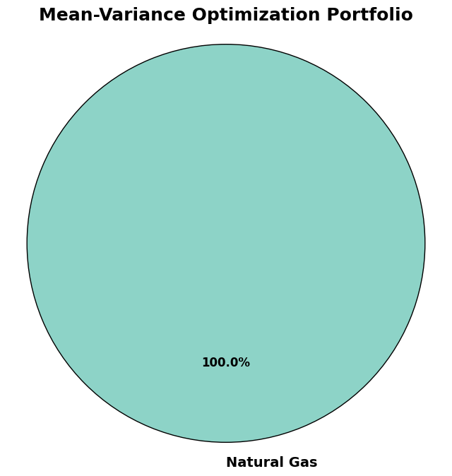
Mean-Variance Optimization: Finds the portfolio with the lowest risk for a given level of return.
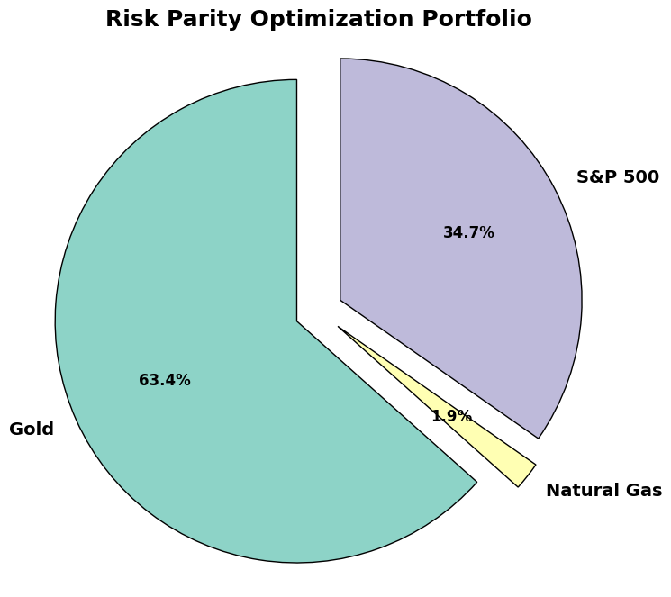
Risk Parity Optimization: Balances risk equally across all assets.
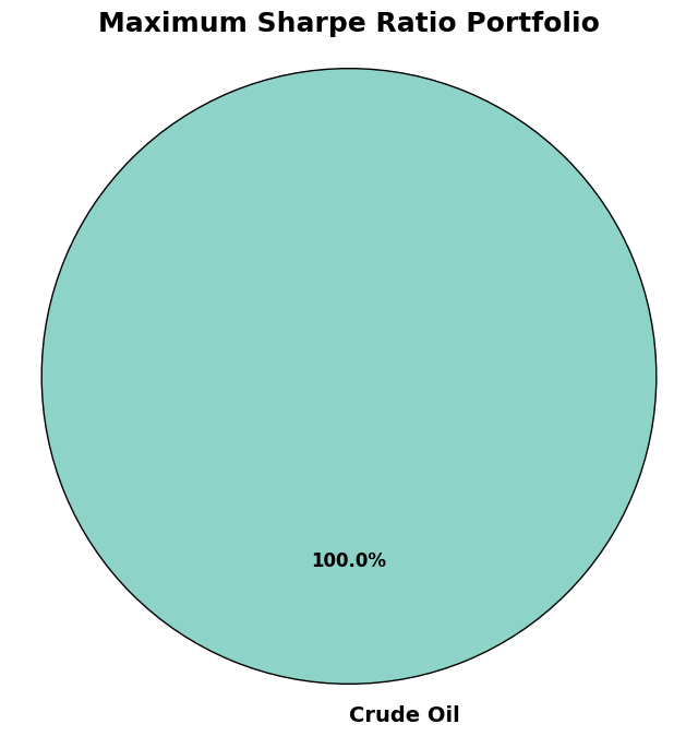
Maximum Sharpe Ratio Optimization: Finds the portfolio with the best risk-adjusted return.
Plot Results:
It creates pie charts to visualize how much money should be invested in each asset based on the optimization results.
Run Optimizations:
It runs each optimization (Mean-Variance, Risk Parity, and Maximum Sharpe Ratio) and displays the results as pie charts.
Outputs#
Mean-Variance Portfolio: A pie chart showing how to distribute investments to minimize risk.
Risk Parity Portfolio: A pie chart showing how to balance risk equally across assets.
Maximum Sharpe Ratio Portfolio: A pie chart showing how to maximize returns relative to risk.
# Install dependencies
%pip install amplpy yfinance matplotlib seaborn pandas numpy requests -q
# Google Colab & Kaggle integration
from amplpy import AMPL, ampl_notebook

ampl = ampl_notebook(
    modules=["gurobi"],  # modules to install
    license_uuid="default",  # license to use
)  # instantiate AMPL object and register magics
Prompt for EIA API key#
You need to provide the API key to be used to fetch data from the EIA (Energy Information Administration) regarding crude oil inventories.
import os
from getpass import getpass

if os.environ.get("EIA_API_KEY", "") == "":
    # Prompt the user to enter their API key securely
    os.environ["EIA_API_KEY"] = getpass("Enter your EIA API key: ")
    print("API Key stored successfully!")
else:
    print("API Key already stored!")
API Key already stored!
Implementation#
Import libraries#
# Import libraries
import yfinance as yf
import pandas as pd
import numpy as np
import matplotlib.pyplot as plt
import seaborn as sns
import requests
Define constants#
# Define commodities and fetch data
COMMODITIES = [
    "CL=F",
    "GC=F",
    "NG=F",
    "SI=F",
    "SPY",
]  # Crude Oil, Gold, Natural Gas, Silver, SPY,

START_DATE = "2020-01-01"
END_DATE = "2025-01-01"
Fetch crude oil inventories from EIA API#
def fetch_crude_inventories(api_key):
    """Fetch crude oil inventories data from EIA API."""
    base_url = "https://api.eia.gov/v2/petroleum/stoc/wstk/data/"
    params = {
        "frequency": "weekly",
        "data[0]": "value",
        "facets[series][]": "WTTSTUS1",
        "sort[0][column]": "period",
        "sort[0][direction]": "desc",
        "offset": 0,
        "length": 5000,
        "api_key": api_key,
    }
    response = requests.get(base_url, params=params)
    if response.status_code == 200:
        data = response.json()
        df = pd.DataFrame(data["response"]["data"])
        df["period"] = pd.to_datetime(df["period"])
        df.set_index("period", inplace=True)
        return df[["value"]].rename(columns={"value": "Inventories"})
    else:
        raise Exception(f"Failed to fetch data: {response.status_code}")
Download historical data for commodities#
def fetch_commodities_data(tickers, start_date, end_date):
    """Fetch historical data for given tickers."""
    data = yf.download(tickers, start=start_date, end=end_date)["Close"]
    return data
Calculate returns and covariance matrix#
def calculate_statistics(data):
    """Calculate daily returns and covariance matrix."""
    returns = data.pct_change(fill_method=None).dropna()
    cov_matrix = returns.cov().values
    mean_returns = returns.mean().values
    return returns, cov_matrix, mean_returns
Plot a pie chart of portfolio weights#
def plot_pie_chart(weights, title):
    """Plot a pie chart of portfolio weights with improved visuals."""

    # Define a dictionary to map tickers to their respective names
    ticker_to_name = {
        "CL=F": "Crude Oil",
        "GC=F": "Gold",
        "NG=F": "Natural Gas",
        "SI=F": "Silver",
        "SPY": "S&P 500",
    }

    # Map the tickers in the portfolio to their actual names
    labels = [ticker_to_name[ticker] for ticker in weights.index]

    # Filter out the tickers with weight less than or equal to 1e-4
    filtered_weights = weights[weights > 1e-4]
    filtered_labels = [
        label
        for label, ticker in zip(labels, weights.index)
        if ticker in filtered_weights.index
    ]

    # Set color palette
    palette = sns.color_palette("Set3", len(filtered_weights))

    # Plot the pie chart
    plt.figure(figsize=(8, 8))
    wedges, texts, autotexts = plt.pie(
        filtered_weights,
        labels=filtered_labels,
        autopct="%1.1f%%",
        startangle=90,
        colors=palette,
        explode=[0.1]
        * len(filtered_weights),  # Slightly "explode" all slices for emphasis
        wedgeprops={"edgecolor": "black", "linewidth": 1, "linestyle": "solid"},
    )

    # Improve text labels
    for text in texts:
        text.set_fontsize(14)
        text.set_fontweight("bold")
    for autotext in autotexts:
        autotext.set_fontsize(12)
        autotext.set_fontweight("bold")

    # Add title
    plt.title(title, fontsize=18, fontweight="bold")

    # Equal aspect ratio ensures that pie is drawn as a circle.
    plt.axis("equal")

    # Show the plot
    plt.show()
Mean-Variance Optimization#
def mean_variance_optimization(tickers, cov_matrix, mean_returns, risk_tolerance):
    """Perform Markowitz mean-variance optimization."""
    ampl = AMPL()
    # Define the AMPL model
    ampl.eval(
        r"""
        set A ordered;  # Set of assets
        param S{A, A};  # Covariance matrix
        param mu{A};    # Expected returns
        param gamma;    # Risk tolerance
        var w{A} >= 0 <= 1;  # Portfolio weights

        maximize expected_return:
            sum {i in A} mu[i] * w[i];  # Objective: maximize expected return

        s.t. portfolio_weights:
            sum {i in A} w[i] = 1;  # Constraint: weights sum to 1

        s.t. risk_constraint:
            sum {i in A, j in A} w[i] * S[i, j] * w[j] <= gamma;  # Risk constraint
    """
    )

    # Set data in AMPL
    ampl.set["A"] = tickers
    ampl.param["S"] = pd.DataFrame(cov_matrix, index=tickers, columns=tickers)
    ampl.param["mu"] = pd.Series(mean_returns, index=tickers)
    ampl.param["gamma"] = risk_tolerance

    # Solve the optimization problem
    ampl.solve(solver="gurobi", mp_options="outlev=1")

    # Extract and return portfolio weights
    return pd.Series(ampl.var["w"].to_dict())
Risk Parity Optimization#
def risk_parity_optimization(tickers, cov_matrix, total_volatility):
    """Perform risk parity optimization."""
    ampl = AMPL()
    # Define the AMPL model
    ampl.eval(
        r"""
        set A ordered;  # Set of assets
        param S{A, A};  # Covariance matrix
        param total_volatility;  # Total portfolio volatility
        var w{A} >= 0 <= 1;  # Portfolio weights

        minimize risk_parity:
            sum {i in A} (w[i] * sum {j in A} S[i, j] * w[j]) / total_volatility;  # Objective: risk parity

        s.t. portfolio_weights:
            sum {i in A} w[i] = 1;  # Constraint: weights sum to 1
        """
    )

    # Set data in AMPL
    ampl.set["A"] = tickers
    ampl.param["S"] = pd.DataFrame(cov_matrix, index=tickers, columns=tickers)
    ampl.param["total_volatility"] = total_volatility

    # Solve the optimization problem
    ampl.solve(solver="gurobi", mp_options="outlev=1")

    # Extract and return portfolio weights
    return pd.Series(ampl.var["w"].to_dict())
Maximum Sharpe Ratio Optimization#
def max_sharpe_optimization(tickers, cov_matrix, mean_returns, risk_free_rate=0.02):
    """Perform maximum Sharpe ratio optimization."""
    ampl = AMPL()
    # Define the AMPL model
    ampl.eval(
        r"""
        set A ordered;  # Set of assets
        param S{A, A};  # Covariance matrix
        param mu{A};  # Mean returns
        param risk_free_rate;  # Risk-free rate
        var w{A} >= 0 <= 1;  # Portfolio weights

        maximize sharpe_ratio:
            (sum {i in A} mu[i] * w[i] - risk_free_rate) /
            sqrt(sum {i in A, j in A} w[i] * S[i, j] * w[j]);  # Objective: maximize Sharpe ratio

        s.t. portfolio_weights:
            sum {i in A} w[i] = 1;  # Constraint: weights sum to 1
        """
    )

    # Set data in AMPL
    ampl.set["A"] = tickers
    ampl.param["S"] = pd.DataFrame(cov_matrix, index=tickers, columns=tickers)
    ampl.param["mu"] = pd.Series(mean_returns, index=tickers).to_dict()
    ampl.param["risk_free_rate"] = risk_free_rate

    # Solve the optimization problem
    ampl.solve(solver="gurobi", mp_options="outlev=1")

    # Extract and return portfolio weights
    return pd.Series(ampl.var["w"].to_dict())
Execution#
Fetch EIA data#
crude_inventories = fetch_crude_inventories(os.environ["EIA_API_KEY"])
commodities_data = fetch_commodities_data(COMMODITIES, START_DATE, END_DATE)
[*********************100%***********************] 5 of 5 completed
Calculate statistics#
returns, cov_matrix, mean_returns = calculate_statistics(commodities_data)
Mean-Variance Optimization#
risk_tolerance = 0.01  # Set risk tolerance (gamma)
mean_variance_weights = mean_variance_optimization(
    COMMODITIES, cov_matrix, mean_returns, risk_tolerance
)
plot_pie_chart(mean_variance_weights, "Mean-Variance Optimization Portfolio")
Gurobi 12.0.1: Set parameter LogToConsole to value 1
  tech:outlev = 1

AMPL MP initial flat model has 5 variables (0 integer, 0 binary);
Objectives: 1 linear;
Constraints:  1 linear; 1 quadratic;

AMPL MP final model has 5 variables (0 integer, 0 binary);
Objectives: 1 linear;
Constraints:  1 linear; 1 quadratic;


Set parameter InfUnbdInfo to value 1
Gurobi Optimizer version 12.0.1 build v12.0.1rc0 (linux64 - "Ubuntu 22.04.4 LTS")

CPU model: Intel(R) Xeon(R) CPU @ 2.20GHz, instruction set [SSE2|AVX|AVX2]
Thread count: 1 physical cores, 2 logical processors, using up to 2 threads

Non-default parameters:
InfUnbdInfo  1

Optimize a model with 1 rows, 5 columns and 5 nonzeros
Model fingerprint: 0xe6499714
Model has 1 quadratic constraint
Coefficient statistics:
  Matrix range     [1e+00, 1e+00]
  QMatrix range    [2e-05, 1e-02]
  Objective range  [5e-04, 2e-03]
  Bounds range     [1e+00, 1e+00]
  RHS range        [1e+00, 1e+00]
  QRHS range       [1e-02, 1e-02]
Presolve time: 0.01s
Presolved: 6 rows, 11 columns, 25 nonzeros
Presolved model has 1 second-order cone constraint
Ordering time: 0.00s

Barrier statistics:
 AA' NZ     : 1.500e+01
 Factor NZ  : 2.100e+01
 Factor Ops : 9.100e+01 (less than 1 second per iteration)
 Threads    : 1

                  Objective                Residual
Iter       Primal          Dual         Primal    Dual     Compl     Time
   0   3.05203426e-04  5.09886629e-04  5.00e-01 8.71e-02  1.96e-02     0s
   1   8.13535516e-04  9.84179460e-04  5.50e-07 4.54e-02  3.50e-03     0s
   2   1.56040833e-03  1.66262088e-03  5.54e-10 1.22e-10  3.85e-04     0s
   3   1.56952131e-03  1.56967543e-03  4.09e-14 1.98e-13  5.80e-07     0s

Barrier solved model in 3 iterations and 0.01 seconds (0.00 work units)
Optimal objective 1.56952131e-03

Warning: to get QCP duals, please set parameter QCPDual to 1
Gurobi 12.0.1: optimal solution; objective 0.001569521313
0 simplex iterations
3 barrier iterations
Risk Parity Optimization#
total_volatility = np.sqrt(np.dot(mean_returns, np.dot(cov_matrix, mean_returns)))
risk_parity_weights = risk_parity_optimization(
    COMMODITIES, cov_matrix, total_volatility
)
plot_pie_chart(risk_parity_weights, "Risk Parity Optimization Portfolio")
Gurobi 12.0.1: Set parameter LogToConsole to value 1
  tech:outlev = 1

AMPL MP initial flat model has 5 variables (0 integer, 0 binary);
Objectives: 1 quadratic;
Constraints:  1 linear;

AMPL MP final model has 5 variables (0 integer, 0 binary);
Objectives: 1 quadratic;
Constraints:  1 linear;


Set parameter InfUnbdInfo to value 1
Gurobi Optimizer version 12.0.1 build v12.0.1rc0 (linux64 - "Ubuntu 22.04.4 LTS")

CPU model: Intel(R) Xeon(R) CPU @ 2.20GHz, instruction set [SSE2|AVX|AVX2]
Thread count: 1 physical cores, 2 logical processors, using up to 2 threads

Non-default parameters:
InfUnbdInfo  1

Optimize a model with 1 rows, 5 columns and 5 nonzeros
Model fingerprint: 0xfcd63839
Model has 15 quadratic objective terms
Coefficient statistics:
  Matrix range     [1e+00, 1e+00]
  Objective range  [0e+00, 0e+00]
  QObjective range [2e-01, 8e+01]
  Bounds range     [1e+00, 1e+00]
  RHS range        [1e+00, 1e+00]
Presolve time: 0.00s
Presolved: 1 rows, 5 columns, 5 nonzeros
Presolved model has 15 quadratic objective terms
Ordering time: 0.00s

Barrier statistics:
 Free vars  : 4
 AA' NZ     : 1.000e+01
 Factor NZ  : 1.500e+01
 Factor Ops : 5.500e+01 (less than 1 second per iteration)
 Threads    : 1

                  Objective                Residual
Iter       Primal          Dual         Primal    Dual     Compl     Time
   0   2.78832253e+06 -2.78832253e+06  2.54e+03 6.79e-07  2.70e+05     0s
   1   9.30586873e+04 -9.46563498e+04  2.01e+02 5.36e-08  2.36e+04     0s
   2   3.79456521e+03 -6.31951849e+03  7.73e+00 2.06e-09  1.03e+03     0s
   3   1.37694437e+01 -2.68239094e+03  7.73e-06 1.26e-13  3.37e+01     0s
   4   1.33697286e+01 -1.56986044e+01  5.12e-08 2.22e-16  3.63e-01     0s
   5   1.86487254e+00 -1.10618752e+01  5.12e-14 1.75e-15  1.62e-01     0s
   6   7.58098847e-01 -7.66313473e-02  2.78e-16 5.55e-17  1.04e-02     0s
   7   3.73429178e-01  2.50225031e-01  5.55e-17 1.11e-16  1.54e-03     0s
   8   3.15925444e-01  3.01868511e-01  2.78e-17 6.94e-17  1.76e-04     0s
   9   3.09299458e-01  3.07418093e-01  6.11e-16 2.78e-17  2.35e-05     0s
  10   3.08303061e-01  3.08054827e-01  1.72e-15 1.39e-17  3.10e-06     0s
  11   3.08129206e-01  3.08107080e-01  1.33e-14 2.78e-17  2.77e-07     0s
  12   3.08108678e-01  3.08108472e-01  1.63e-14 5.55e-17  2.58e-09     0s
  13   3.08108474e-01  3.08108474e-01  2.81e-14 3.47e-18  2.58e-12     0s

Barrier solved model in 13 iterations and 0.00 seconds (0.00 work units)
Optimal objective 3.08108474e-01

Gurobi 12.0.1: optimal solution; objective 0.308108474
0 simplex iterations
13 barrier iterations
Max Sharpe Optimization#
# Maximum Sharpe Ratio Optimization
max_sharpe_weights = max_sharpe_optimization(COMMODITIES, cov_matrix, mean_returns)
plot_pie_chart(max_sharpe_weights, "Maximum Sharpe Ratio Portfolio")
Gurobi 12.0.1: Set parameter LogToConsole to value 1
  tech:outlev = 1

AMPL MP initial flat model has 5 variables (0 integer, 0 binary);
Objectives: 1 linear;
Constraints:  2 linear; 1 quadratic;
Algebraic expressions:  1 div; 1 powconstexp;

AMPL MP final model has 9 variables (0 integer, 0 binary);
Objectives: 1 linear;
Constraints:  2 linear; 1 quadratic;
Algebraic expressions:  1 div; 1 powconstexp;


Set parameter InfUnbdInfo to value 1
Gurobi Optimizer version 12.0.1 build v12.0.1rc0 (linux64 - "Ubuntu 22.04.4 LTS")

CPU model: Intel(R) Xeon(R) CPU @ 2.20GHz, instruction set [SSE2|AVX|AVX2]
Thread count: 1 physical cores, 2 logical processors, using up to 2 threads

Non-default parameters:
InfUnbdInfo  1

Optimize a model with 1 rows, 9 columns and 5 nonzeros
Model fingerprint: 0x2dd5ab5a
Model has 1 general nonlinear constraint (17 nonlinear terms)
Variable types: 9 continuous, 0 integer (0 binary)
Coefficient statistics:
  Matrix range     [1e+00, 1e+00]
  Objective range  [1e+00, 1e+00]
  Bounds range     [8e-05, 1e+00]
  RHS range        [1e+00, 1e+00]
Presolve model has 1 nlconstr
Added 33 variables to disaggregate expressions.
Presolve removed 0 rows and 3 columns
Presolve time: 0.00s
Presolved: 82 rows, 40 columns, 182 nonzeros
Presolved model has 16 bilinear constraint(s)
Presolved model has 1 nonlinear constraint(s)

Solving non-convex MINLP

Variable types: 40 continuous, 0 integer (0 binary)
Found heuristic solution: objective -0.2237351

Root relaxation: interrupted, 20 iterations, 0.00 seconds (0.00 work units)

    Nodes    |    Current Node    |     Objective Bounds      |     Work
 Expl Unexpl |  Obj  Depth IntInf | Incumbent    BestBd   Gap | It/Node Time

     0     0          -    0        -0.22374   -0.22372  0.01%     -    0s

Explored 1 nodes (20 simplex iterations) in 0.01 seconds (0.00 work units)
Thread count was 2 (of 2 available processors)

Solution count 1: -0.223735

Optimal solution found (tolerance 1.00e-04)
Best objective -2.237350923262e-01, best bound -2.237198990814e-01, gap 0.0068%
Gurobi 12.0.1: optimal solution; objective -0.2237350923
20 simplex iterations
1 branching node
absmipgap=1.51932e-05, relmipgap=6.79073e-05