
Power Generation Portfolio Optimization#
![]()
![]()


![]()

Description: Power generation portfolio optimization to manage several assets and resources.
Tags: amplpy, energy, power generation, Electric Power Industry
Notebook author: Juan Pablo Bohórquez <juan@ampl.com>
Model author: Juan Pablo Bohórquez <juan@ampl.com>
# Install dependencies
%pip install -q amplpy pandas matplotlib openpyxl ipywidgets
# Google Colab & Kaggle integration
from amplpy import AMPL, ampl_notebook

ampl = ampl_notebook(
    modules=["highs"],  # modules to install
    license_uuid="default",  # license to use
)  # instantiate AMPL object and register magics
1. Problem Description#
In liberalized electricity markets, generation companies face a complex daily challenge: how to operate a diverse fleet of power plants to maximize profit without violating physical or environmental constraints. It is not uncommon for large market participants to own a portfolio of several power generation technologies (e.g. big hydro with reservoirs, small run-of-river hydro, solar, wind, thermal plants, batteries, among others) and correctly managing them is not a trivial task. This problem is refered to as Power Generation Portfolio Optimization. The objective is to maximize Producer Surplus, defined mathematically as the difference between the revenue gained from selling energy at market prices and the variable costs of production (fuel and operations).
The challenge lies in managing the several assets with their own competing characteristics. Firstly, thermal units (coal, gas, nuclear) provide stable baseload power but come with high marginal costs and physical inertia. They consume fuel for every MWh produced and cannot change output instantly. The model should account for ramp constraints, forcing the optimizer to “plan ahead” for peak price hours rather than reacting instantly. On the other hand, hydropower is the most complex asset to manage because it can affect both time and space dimensions. Time is coupled through reservoirs where one can store water (energy) today to use in the future. Besides that, rivers often have multiple generators in a chain. In this sense, water released from an “Upstream” dam flows down to become inflow for a “Downstream” one. This creates a dependency where the generation of one unit affects the resource availability of another. Finally, renewables like solar and wind are zero-marginal-cost resources whose energy, ideally, must be produced whenever it is available.
Throughout this notebook reservoir and dam are used indistinctively.
1.1 Simplifications#
The model that will be presented below has some simplifications made that are crucial to understand its results:
The model is explicitly intended to be a linear program, in order to make it easy to solve by any LP engine. This means that binary variables are avoided wherever possible. Thus, model’s capacity to include some unit-commitment constraints such as startup/shutdown costs is limited.
It is assumed that the market where the generation firm is participating is a competitive one. This implies, by definition, that all agents are price takers and their particular generation should not alter the market price. This assumption is key, otherwise the model would be non-linear and much harder to solve.
Hydraulic cascades are modeled but the only valid topology is the one where upstream plants turbine and spill to the downstream one. More complex configurations are found in real systems and may be modeled using explicit sets segementation. However, for the sake of simplicity this is not modeled.
The efficiency of reservoir hydro plants (the conversion factor by which they convert water into energy - \([MW/m^3/s]\)) is assumed to be constant. A more detailed approach would be to model it as a piecewise-linear function depending on the dam level. This would require binary variables that, as mentioned before, are being simplified for this base case.
The agent will always be able to produce as much as it needs with its intermittent renewable sources. This is not necesarily the case in all electricity markets. Should the installed capacity of the system be large enough or due to some grid constraints, agent generation may be curtailed. Some of this should be incorporated in the market price (e.g. an excess in capacity can make the price go to zero), other bits may have to be included in the forecasted resource that’ll limit the maximum generation of these plants.
2. Model#
This section provides a mathematical description of the model with their AMPL counter parts as they are created in a later cell.
2.1 Sets and Indices#
Symbol |
Description |
AMPL Code Equivalent |
|---|---|---|
\(t \in {T}\) |
Set of time periods (hours), indexed \(1..T\). |
|
\(g \in G\) |
Set of all generators. |
|
\(G^{Therm} \subset G\) |
Set of thermal generators (e.g., Gas, Coal). |
|
\(G^{Hydro} \subset G\) |
Set of all hydro generators. |
|
\(G^{Res} \subset G^{Hydro}\) |
Hydro generators with reservoir storage. |
|
\(G^{RoR} \subset G^{Hydro}\) |
Run-of-River hydro generators (no storage). |
|
\(G^{Ren} \subset G\) |
Renewable generators (Solar \(\cup\) Wind). |
|
\(U_g \subset G^{Hydro}\) |
Set of generators immediately upstream of unit \(g\). |
|
2.2 Parameters#
Symbol |
Description |
Unit |
AMPL Parameter |
|---|---|---|---|
\(\pi_t\) |
Forecasted market price at time \(t\) |
$/MWh |
|
\(c_{g,t}\) |
Marginal fuel cost for thermal unit \(g\) at time \(t\) |
$/MWh |
|
\(\rho_g\) |
Penalty cost for water spillage for hydro unit \(g\) |
$/MWh |
|
\(I_{g,t}\) |
Natural exogenous inflows to unit \(g\) at time \(t\) |
\(m^3/s\) |
|
\(\eta_g\) |
Efficiency (water-to-power conversion) for unit \(g\) |
\(MW / (m^3/s)\) |
|
\(V^{max}_g\) |
Maximum reservoir capacity |
\(Hm^3\) |
|
\(V^{init}_g\) |
Initial reservoir storage level at \(t=0\) |
\(Hm^3\) |
|
\(V^{final}_g\) |
Required target storage level at \(t=T\) |
\(Hm^3\) |
|
\(\Delta t\) |
Conversion factor (flow rate to volume) |
- |
|
\(P^{max}_{g,t}\) |
Maximum power generation capacity |
\(MW\) |
|
\(P^{min}_{g,t}\) |
Minimum power generation requirement |
\(MW\) |
|
\(RU_g\) |
Ramp-up rate limit for thermal unit \(g\) |
\(MW/h\) |
|
\(RD_g\) |
Ramp-down rate limit for thermal unit \(g\) |
\(MW/h\) |
|
\(R_{g,t}\) |
Available renewable resource forecast (Solar/Wind) |
\(MW\) |
|
2.3 Decision Variables#
Symbol |
Description |
Unit |
AMPL Variable |
|---|---|---|---|
\(p_{g,t}\) |
Power generation output |
\(MW\) |
|
\(v_{g,t}\) |
Reservoir storage volume at end of period \(t\) |
\(Hm^3\) |
|
\(q_{g,t}\) |
Water flow through the turbines |
\(m^3/s\) |
|
\(\sigma_{g,t}\) |
Water flow spilled (bypassing turbines) |
\(m^3/s\) |
|
\(s_{g,t}\) |
Energy equivalent of spilled water (for accounting) |
\(MWh\) |
|
2.4 Objective Function#
The objective is to maximize Producer Surplus (Total Profit), calculated as Market Revenue minus Variable Costs minus Spillage Penalties.
2.5 Constraints#
2.5.1 Reservoir Hydraulic Balance#
Tracks the conservation of mass for water in reservoirs. The volume at the end of period \(t\) is the previous volume plus total inflows (natural + upstream releases) minus total outflows (turbining + spillage). The constant \(\Delta t\) is used to convert from flow units (\(m^3/s\)) to volume (\(Hm^3\))
(Note: For \(t=1\), \(v_{g,t-1}\) is defined by the parameter \(V^{init}_g\))
2.5.2 Run-of-River (RoR) Balance#
RoR units have no storage capacity. The total water leaving the unit (turbined + spilled) cannot exceed the natural inflow at that moment.
2.5.3 Hydro Production Function#
Defines the linear relationship between water flow and power generation.
2.5.4 Spillage Energy Definition#
Calculates the energy equivalent of spilled water. This variable allows the objective function to penalize spillage in $/MWh terms. Since dam efficiency is assumed to be a constant value, it is also used for this equation.
2.5.5 Reservoir Limits#
Ensures storage never exceeds capacity and meets the end-of-horizon target requirements.
2.5.6 Thermal Ramping Limits#
Constrains the change in power output between consecutive periods to respect the mechanical limits of thermal generators. For simplicity, no initial conditions are considered (i.e. the constraint only applies from the second period onwards).
2.5.7 Generator Output Limits#
Enforces minimum and maximum generation limits.
For renewables, the upper limit is determined by the resource availability (solar/wind forecast). In the case of RoR plants, inflows determine the upper limit of generation. Thus, some caution is advised when passing resource forecasts to the model: they must be limited by each plants capacity.
Note that this step can be avoided by defining a maximum generation constraint for all the generators and not only the conventional ones. This was not done in this notebook, due to data availability. Nevertheless, the change would be trivial in the AMPL code.
Finally, several real operation conditions may be modeled through these constraints. For instance, maintenance maintenance scheduling can be included in the maximum generation constraint. Additional, enviromental or regualtory limits can be modeled using the constraints presented in this section
2.6 AMPL Implementation#
The model explained above is implemented using AMPL in this section.
%%writefile generation_portfolio.mod
# Model Name: Energy Portfolio Optimization (pricetaker)

### SETS
set PERIODS ordered;  # hours
set THERMAL_GENERATORS default {};
set RESERVOIR_HYDRO_GENERATORS default {};
set CONVENTIONAL_GENERATORS = THERMAL_GENERATORS union RESERVOIR_HYDRO_GENERATORS;
set ROR_HYDRO_GENERATORS default {};
set HYDRO_GENERATORS = RESERVOIR_HYDRO_GENERATORS union ROR_HYDRO_GENERATORS;
set UPSTREAM_GENERATORS {HYDRO_GENERATORS} within HYDRO_GENERATORS default {};
set SOLAR_GENERATORS default {};
set WIND_GENERATORS default {};
set RENEWABLE_GENERATORS = SOLAR_GENERATORS union WIND_GENERATORS;
set GENERATORS = THERMAL_GENERATORS union HYDRO_GENERATORS union RENEWABLE_GENERATORS;


### PARAMETERS
# Forecasted Params
param market_price {PERIODS} >= 0;                # Forecasted market energy price ($/MWh)
param marginal_cost {THERMAL_GENERATORS, PERIODS} >= 0;    # Marginal fuel cost ($/MWh)
param inflows {HYDRO_GENERATORS, PERIODS} >= 0 default 0;  # Water contributions/inflows (m3/s)
param renewable_resource {RENEWABLE_GENERATORS, PERIODS} >= 0; # Renewable resource availability (MW)

# Thermal Units Params
param ramp_up_rate {THERMAL_GENERATORS} >= 0;     # Ramp up limit (MW/hour)
param ramp_down_rate {THERMAL_GENERATORS} >= 0;   # Ramp down limit (MW/hour)

# Hydro Params
param efficiency {HYDRO_GENERATORS} > 0;               # Conversion Factor (MW/m3/s)
param reservoir_max_capacity {RESERVOIR_HYDRO_GENERATORS} >= 0; # Reservoir max capacity (Hm3)
param initial_storage {r in RESERVOIR_HYDRO_GENERATORS} >= 0 default 0.7*reservoir_max_capacity[r];         # Initial reservoir energy (Hm3)
param final_storage {r in RESERVOIR_HYDRO_GENERATORS} >= 0 default initial_storage[r];  # Required energy at end of horizon (Hm3)

# Operational Params/Limits
param max_generation {CONVENTIONAL_GENERATORS, PERIODS} >= 0;  # Maximum generation (MW)
param min_generation {GENERATORS, PERIODS} >= 0 default 0;  # Minimum generation (MW)

# Penalty Params
param penalty_spillage {HYDRO_GENERATORS} >= 0 default 2.5* max{t in PERIODS}(market_price[t]); # Penalty for water spillage ($/MWh)

# Computed/Scalar Params
param period_duration >=0 default 3600; # Duration of each period in seconds (default: 1 hour)
param delta_t = period_duration / 1000000;  # Constant to convert m3/s to Hm3 per period


### VARIABLES
var Generation {GENERATORS, PERIODS} >= 0;  # MW
var ReservoirStorage {RESERVOIR_HYDRO_GENERATORS, PERIODS} >= 0;  # Hm3
var TurbiningFlow {HYDRO_GENERATORS, PERIODS} >= 0;  # m3/s
var Spillage {HYDRO_GENERATORS, PERIODS} >= 0;  # MWh
var SpillageFlow {HYDRO_GENERATORS, PERIODS} >= 0;  # m3/s


### OBJECTIVE FUNCTION
maximize TotalProfit:
    sum {g in GENERATORS, t in PERIODS} (market_price[t] * Generation[g, t])
    - sum {g in THERMAL_GENERATORS, t in PERIODS} (marginal_cost[g, t] * Generation[g, t])
    - sum {g in HYDRO_GENERATORS, t in PERIODS} (penalty_spillage[g] * Spillage[g, t]);


### CONSTRAINTS
subject to ReservoirHydroBalance {g in RESERVOIR_HYDRO_GENERATORS, t in PERIODS}:
    ReservoirStorage[g, t] = (if t = first(PERIODS) then initial_storage[g] else ReservoirStorage[g, prev(t)])
                                + delta_t * (inflows[g, t]
                                            + sum {ug in UPSTREAM_GENERATORS[g]} (TurbiningFlow[ug, t] + SpillageFlow[ug, t])
                                            - TurbiningFlow[g, t]
                                            - SpillageFlow[g, t]);

subject to RunOfRiverBalance {g in ROR_HYDRO_GENERATORS, t in PERIODS}:
    TurbiningFlow[g, t] + SpillageFlow[g, t] <= inflows[g, t];

subject to ReservoirStorageLimit {g in RESERVOIR_HYDRO_GENERATORS, t in PERIODS}:
    ReservoirStorage[g, t] <= reservoir_max_capacity[g];

subject to ReservoirFinalStorage {g in RESERVOIR_HYDRO_GENERATORS}:
    ReservoirStorage[g, last(PERIODS)] = final_storage[g];

subject to HydroGenerationFromFlow {g in HYDRO_GENERATORS, t in PERIODS}:
    Generation[g, t] = efficiency[g] * TurbiningFlow[g, t];

subject to HydroSpillageFromFlow {g in HYDRO_GENERATORS, t in PERIODS}:
    Spillage[g, t] = efficiency[g] * SpillageFlow[g, t];

subject to RenewableGenerationLimit {g in RENEWABLE_GENERATORS, t in PERIODS}:
    Generation[g, t] <= renewable_resource[g, t];

subject to ThermalRampUp {g in THERMAL_GENERATORS, t in PERIODS: ord(t) > 1}:
    Generation[g, t] - Generation[g, prev(t)] <= ramp_up_rate[g];

subject to ThermalRampDown {g in THERMAL_GENERATORS, t in PERIODS: ord(t) > 1}:
    Generation[g, prev(t)] - Generation[g, t] <= ramp_down_rate[g];

subject to GenerationMaxLimit {g in CONVENTIONAL_GENERATORS, t in PERIODS}:
    Generation[g, t] <= max_generation[g, t];

subject to GenerationMinLimit {g in GENERATORS, t in PERIODS}:
    Generation[g, t] >= min_generation[g, t];
Overwriting generation_portfolio.mod
3. Data & Scenarios#
3.1 AMPL Default Values#
Several components in the AMPL model utilize default values. These act as logical assumptions to ensure the model solves even if specific data points are missing from the input files, or to establish standard operational baselines.
Set Initializaiton: most sets are initialized to an empty space {}.
Reasoning: keeping the generator sets flexible allows the model to be tested under different portfolio compositions without breaking the code. Thu, model can be used, for instance, to evaluate the impact of a new plant in the portfolio, among other uses.
Initial Storage (\(V^{init}_g\)): Defaults to \(0.7 \times V^{max}_g\).
Reasoning: If specific starting conditions are unknown, we assume reservoirs are at 70% capacity. This provides a neutral starting point—neither empty (risk of shortages) nor full (risk of immediate spillage), allowing the optimizer flexibility in both directions.
Final Storage (\(V^{final}_g\)): Defaults to \(V^{init}_g\).
Reasoning: This imposes a “cyclic” or sustainable operation constraint. It prevents the model from artificially inflating profit by draining the reservoirs dry by the last hour.
Spillage Penalty (\(\rho_g\)): Defaults to \(2.5 \times \max(\pi_t)\).
Reasoning: This is a “soft constraint.” The penalty is set significantly higher than the highest market price to ensure spillage only occurs when physically unavoidable (e.g., reservoirs are full and inflows are high).
3.2 Data Description#
The datasets provided in this repository are grounded in reality to ensure the portfolio optimization results are meaningful.
Portfolio Topology: The generation assets (Thermal, Hydro, Solar, Wind) are based on a real-world energy portfolio from an actual power system. The hydraulic topology (upstream/downstream relationships) reflects real river chains.
Historical Inputs: The time-series data—specifically Market Prices (\(\pi_t\)), Hydrological Inflows (\(I_{g,t}\)), and Renewable Availability (\(R_{g,t}\))—are drawn from historical records across different years. This diversity allows us to test the model’s robustness under various conditions, such as “Dry Years” (low hydro, high prices) vs. “Wet Years” (high hydro, low prices).
The example power generation portfolio studied in this notebook consists of the following plants:
3 reservoir hydro plants. Two of them are chained (i.e. they use the same river and one turbinates and spill water to the other).
8 run-of-river plants.
4 thermal generators.
Up to 4 solar plants (depending on the scenario).
The time horizon of each scenario is 1 year, with hourly periods. This means each scenario implies a LP model with roughly ~480.000 variables and ~650.000 constraints. Since the size of the model is greater than the free tier limitation of most commercial solvers, an open-source solver will be used used instead (i.e. Highs).
3.3 Repository File Naming#
To facilitate batch processing and scenario analysis, the data and results follow a strict naming convention. All files are accesible in the repository.
Inputs:
data_S{x}.xlsxandtechnical_data.xlsxContains all the input data for Scenario x (e.g.,
data_S1.xlsx,data_S2.xlsx).The technical data file includes parameters such as ramps, efficiency and reservoir capacity.
Outputs:
results_S{x}.xlsxThe optimization results for Scenario x are automatically exported to this file after the model solves, for further processing.
Snapshots:
model_snapshot_S{x}.runAMPL session snapshots for each scenario run are saved in case they want to be loaded later for further analysis and testing.
4. Code#
Given that multiple scenarios will be solved and analysed, code is wrapped with some auxiliary python functions that allow to solve the problem and create a dashboard that’ll be presented in the following sections. The general code flow follows these steps:
Read the model file.
Read the data.
Load data into the model.
Solve using specific AMPL options or solver parameters.
Export model.
Fetch solution or manage optimization result.
Export results and analyse.
In order to complete these steps, several amplpy functionalities are used. For instance, data is loaded using the native support of pandas data structures, and the snapshot feature is used to export complete model (with data and options). Moreover, data is extracted and transformed taking advantage of AMPL’s intuitive syntax.
4.1 Implementation#
4.1.1 Libraries#
import pandas as pd
from collections import defaultdict
import ipywidgets as widgets
from IPython.display import display
import matplotlib.pyplot as plt
4.1.2 Optimization Functions#
def load_data_to_model(ampl, scenario="S1"):
    """
    Load input data from Excel files and populate the AMPL model with sets and parameters.

    Parameters:
        ampl (AMPL): The AMPL object to load data into.
        scenario (str): Scenario identifier (default: 'S1'). Used to locate data_S{scenario}.xlsx file.

    Returns:
        None. Modifies the ampl object in-place by loading sets and parameters.

    Raises:
        FileNotFoundError: If data_{scenario}.xlsx or technical_data.xlsx files are not found.
        KeyError: If expected sheet names or columns are missing from the Excel files.

    Notes:
        - Assumes Excel files follow the naming convention: data_S{scenario}.xlsx and technical_data.xlsx
        - Automatically rounds all numeric values to 4 decimal places to avoid numerical issues in solver
        - Generator naming conventions are used to derive additional sets:
          * Hydro generators containing 'ror' are classified as run-of-river
          * Renewable generators containing 'solar' are solar units
          * Renewable generators containing 'wind' are wind units
        - Hydro cascade topology (upstream relationships) must be manually specified after function call
    """
    scenario_file = f"https://raw.githubusercontent.com/ampl/colab.ampl.com/master/authors/jpbohorquez/generation_portfolio/data_{scenario}.xlsx"
    technical_data_file = "https://raw.githubusercontent.com/ampl/colab.ampl.com/master/authors/jpbohorquez/generation_portfolio/technical_data.xlsx"

    dct_data = pd.read_excel(scenario_file, sheet_name=None)
    dct_data = {
        k: v.round(4) for k, v in dct_data.items()
    }  # Rounding to avoid numercal issues

    dct_technical = pd.read_excel(technical_data_file, sheet_name=None)
    dct_technical = {
        k: v.round(4) for k, v in dct_technical.items()
    }  # Rounding to avoid numercal issues

    # region: Processing Data

    # Technical Data
    ramps = dct_technical["ramps"].set_index(
        "thermal_gen"
    )  # Defines set of THERMAL_GENERATORS
    efficiency = dct_technical["efficiency"].set_index("hydro_gen")
    reservoir_cap = dct_technical["reservoir_cap"].set_index(
        "hydro_gen"
    )  # Defines set of RESERVOIR_HYDRO_GENERATORS

    # Scenario Data
    market_price = dct_data["market_price"].set_index(
        "period"
    )  # Defines set of PERIODS
    marginal_cost = dct_data["marginal_cost"].set_index(["thermal_gen", "period"])
    inflows = dct_data["inflows"].set_index(["hydro_gen", "period"])
    renewable_resource = dct_data["renewable_resource"].set_index(
        ["renewable_gen", "period"]
    )
    max_generation = dct_data["max_generation"].set_index(["con_gen", "period"])

    # Additional Sets (takes advantage of naming conventions)
    ROR_HYDRO_GENERATORS = [
        gen for gen in dct_technical["efficiency"]["hydro_gen"].unique() if "ror" in gen
    ]
    SOLAR_GENERATORS = [
        gen
        for gen in dct_data["renewable_resource"]["renewable_gen"].unique()
        if "solar" in gen
    ]
    WIND_GENERATORS = [
        gen
        for gen in dct_data["renewable_resource"]["renewable_gen"].unique()
        if "wind" in gen
    ]

    # endregion

    # region: Loading Data to AMPL Model
    # Sets
    ampl.set["ROR_HYDRO_GENERATORS"] = ROR_HYDRO_GENERATORS
    ampl.set["SOLAR_GENERATORS"] = SOLAR_GENERATORS
    ampl.set["WIND_GENERATORS"] = WIND_GENERATORS

    # Sets and Params
    ampl.set_data(ramps, set_name="THERMAL_GENERATORS")
    ampl.set_data(reservoir_cap, set_name="RESERVOIR_HYDRO_GENERATORS")
    ampl.set_data(market_price, set_name="PERIODS")

    # Additional Sets (hydro topology)
    upstream_set_collection = ampl.set["UPSTREAM_GENERATORS"]
    upstream_set_collection["reservoir1"] = ["reservoir3"]

    # Additional Params
    ampl.set_data(efficiency)
    ampl.set_data(marginal_cost)
    ampl.set_data(inflows)
    ampl.set_data(renewable_resource)
    ampl.set_data(max_generation)
    # endregion


def solve_model(ampl, scenario="S1", export_model=False, verbose=False, **kwargs):
    """
    Solve the generation portfolio optimization model for a given scenario.

    Parameters:
        ampl (AMPL): The AMPL object containing the model.
        scenario (str): Scenario identifier (default: 'S1'). Used to locate data_S{scenario}.xlsx file.
        export_model (bool): If True, exports model snapshot to model_snapshot_{scenario}.run (default: True).
        verbose (bool): If True, prints solver output (default: False).
        **kwargs: Additional AMPL options to set before solving (e.g., solver='highs', presolve=0).

    Returns:
        None. Modifies the ampl object in-place, solves the model, and exports model snapshot if requested.

    Raises:
        FileNotFoundError: If generation_portfolio.mod, data_{scenario}.xlsx, or technical_data.xlsx files are not found.
        RuntimeError: If the solver fails or the model is infeasible/unbounded.

    Notes:
        - Resets the AMPL environment before loading the model to ensure a clean state
        - Requires generation_portfolio.mod to be in the working directory
        - Automatically loads sets and parameters via load_data_to_model()
        - Prints total profit to console if model solves successfully
        - Exports model snapshot if export_model=True
    """
    ampl.reset()
    ampl.read("generation_portfolio.mod")

    load_data_to_model(ampl, scenario=scenario)

    ampl.eval("reset options;")
    for k, v in kwargs.items():
        ampl.set_option(k, v)
    ampl.solve(verbose=verbose)

    if ampl.solve_result == "solved":
        objective = ampl.get_objective("TotalProfit").value()
        print(f"Total Profit ({scenario}): {round(objective/1e6, 2)} MUSD.")
    else:
        print(f"Optimization failed with status: {ampl.solve_result}")

    if export_model:
        ampl.snapshot(f"model_snapshot_{scenario}.run")
        print("Model snapshot exported.")


def process_results(ampl, scenario="S1", export_results=False):
    """
    Process and export the results of the solved AMPL model for a given scenario.

    Parameters:
        ampl (AMPL): The AMPL object containing the solved model.
        scenario (str): Scenario identifier (default: 'S1'). Used to name the exported results file.
        export_results (bool): If True, exports results to results_{scenario}.xlsx (default: False).

    Returns:
        tuple: A tuple containing:
            - df_thermal (pd.DataFrame): DataFrame with marginal costs for thermal generators.
            - df_gen (pd.DataFrame): DataFrame with generation values for all generators.
            - df_dams (pd.DataFrame): DataFrame with reservoir storage, inflows, spillage, and dual values for hydro generators.
            - df_sys (pd.DataFrame): DataFrame with market prices for each period.

    Raises:
        RuntimeError: If the model has not been solved or the solution is not available.

    Notes:
        - Assumes the model has been solved successfully before calling this function.
        - Exports results to an Excel file if export_results=True.
        - The results DataFrames are indexed appropriately based on their content.
    """

    if ampl.solve_result == "solved":
        results_df = pd.DataFrame.from_dict(ampl.get_solution(flat=False, zeros=False))
        results_df = results_df.reset_index(names=["gen", "period"])

        if export_results:
            results_df.to_excel(f"results_{scenario}.xlsx", index=False)
            print(f"Results exported to results_{scenario}.xlsx")

        df_thermal = (
            ampl.get_data("marginal_cost")
            .to_pandas()
            .reset_index(names=["gen", "period"])
        )
        df_thermal.columns = ["gen", "period", "MarginalCost [$/MWh]"]
        df_thermal["scenario"] = scenario

        df_gen = (
            ampl.get_data("Generation").to_pandas().reset_index(names=["gen", "period"])
        )
        df_gen.columns = ["gen", "period", "Generation [MWh]"]
        df_gen["scenario"] = scenario

        dams_indexer = "{g in RESERVOIR_HYDRO_GENERATORS, t in PERIODS}"
        df_dams = (
            ampl.get_data(
                f""" {dams_indexer} ReservoirStorage[g,t]/reservoir_max_capacity[g],
                                    {dams_indexer} ReservoirHydroBalance.dual[g,t] * delta_t / efficiency[g]
                                """
            )
            .to_pandas()
            .reset_index(names=["gen", "period"])
        )
        df_dams.columns = [
            "gen",
            "period",
            "NormalizedReservoirStorage [p.u.]",
            "WaterValue [$/MWh]",
        ]
        df_dams["scenario"] = scenario

        df_hydro = (
            ampl.get_data(
                f""" inflows,
                                    Spillage
                                """
            )
            .to_pandas()
            .reset_index(names=["gen", "period"])
        )
        df_hydro.columns = ["gen", "period", "Inflows [m3/s]", "Spillage [MWh]"]
        df_hydro["scenario"] = scenario

        df_sys = ampl.get_data("market_price").to_pandas().reset_index(names=["period"])
        df_sys.columns = ["period", "MarketPrice [$/MWh]"]
        df_sys["scenario"] = scenario

        df_technical = (
            ampl.get_data(
                "{g in RESERVOIR_HYDRO_GENERATORS} efficiency[g], reservoir_max_capacity"
            )
            .to_pandas()
            .reset_index(names=["gen"])
        )
        df_technical.columns = [
            "gen",
            "Efficiency [MW/m3/s]",
            "ReservoirMaxCapacity [Hm3]",
        ]
        df_technical["scenario"] = scenario

        return df_thermal, df_gen, df_dams, df_hydro, df_sys, df_technical
    else:
        return None, None, None, None, None, None
4.1.3 Plotting Functions#
def plot_dual_axis(left_series, right_series, title=""):
    """
    Helper function for dual-axis plotting.
    Args:
        left_series: List of dicts {'x': ..., 'y': ..., 'label': ..., 'color': ...}
        right_series: List of dicts {'x': ..., 'y': ..., 'label': ..., 'color': ...}
    """
    fig, ax1 = plt.subplots(figsize=(12, 6), layout="tight")

    # Plot Left Axis Series
    for s in left_series:
        ax1.plot(s["x"], s["y"], label=s["label"], color=s.get("color"), linewidth=2)

    ax1.set_xlabel("Period")
    # Use the label of the first item as the axis label if only one, else generic
    left_label = left_series[0]["label"] if len(left_series) == 1 else "Left Axis"
    left_color = (
        left_series[0].get("color", "black") if len(left_series) == 1 else "black"
    )

    ax1.set_ylabel(left_label, color=left_color, fontweight="bold")
    ax1.tick_params(axis="y", labelcolor=left_color)
    ax1.grid(True, alpha=0.3)
    ax1.legend(loc="upper left")

    # Plot Right Axis Series
    if right_series:
        ax2 = ax1.twinx()
        for s in right_series:
            # Use dashed lines for right axis to distinguish
            ax2.plot(
                s["x"],
                s["y"],
                label=s["label"],
                color=s.get("color"),
                linestyle="--",
                linewidth=2,
            )

        right_label = (
            right_series[0]["label"] if len(right_series) == 1 else "Right Axis"
        )
        right_color = (
            right_series[0].get("color", "black") if len(right_series) == 1 else "black"
        )

        ax2.set_ylabel(right_label, color=right_color, fontweight="bold")
        ax2.tick_params(axis="y", labelcolor=right_color)
        ax2.grid(False)

        # Combine legends
        lines1, labels1 = ax1.get_legend_handles_labels()
        lines2, labels2 = ax2.get_legend_handles_labels()
        ax1.legend(lines1 + lines2, labels1 + labels2, loc="upper left")

    ax1.set_title(title, fontweight="bold")

    return fig


def plot_simple_variable(
    results, variable, scenarios, generators=[], granularity="Hourly", agg_func="mean"
):
    # Determine which dataframe to use
    if variable in results["df_gen"].columns:
        df = results["df_gen"]
    elif variable in results["df_dams"].columns:
        df = results["df_dams"]
    elif variable in results["df_hydro"].columns:
        df = results["df_hydro"]
    elif variable in results["df_sys"].columns:
        df = results["df_sys"]
    elif variable in results["df_thermal"].columns:
        df = results["df_thermal"]
    else:
        print(f"Variable '{variable}' not found in results.")
        return

    # Filter data
    mask = (
        (df["scenario"].isin(scenarios)) & (df["gen"].isin(generators))
        if generators
        else (df["scenario"].isin(scenarios))
    )
    data = df[mask].copy()

    if data.empty:
        print("No data found for the selected filters.")
        return

    # Handle Granularity
    if granularity == "Daily":
        data["group_period"] = (data["period"] - 1) // 24
    elif granularity == "Monthly":
        data["group_period"] = (data["period"] - 1) // 730  # Approx hours in month
    else:
        data["group_period"] = data["period"]

    # Aggregation
    group_cols = (
        ["scenario", "gen", "group_period"]
        if generators
        else ["scenario", "group_period"]
    )

    if granularity != "Hourly":
        # Select only numeric columns for aggregation to avoid errors with string cols
        numeric_cols = [variable]
        data = data.groupby(group_cols)[numeric_cols].agg(agg_func).reset_index()
        # Rename group_period back to period for plotting consistency
        data.rename(columns={"group_period": "period"}, inplace=True)

    fig, ax = plt.subplots(figsize=(12, 6), layout="tight")

    # Manually group to mimic hue/style behavior
    groups = (
        data.groupby(["scenario", "gen"]) if generators else data.groupby(["scenario"])
    )

    for tup, group in groups:
        scen = tup[0]
        gen = tup[1] if generators else ""
        label = f"{scen} - {gen}" if generators else f"{scen}"
        ax.plot(group["period"], group[variable], label=label)

    ax.set_title(f"{variable} Analysis ({granularity} - {agg_func})")
    ax.set_xlabel(granularity + " Period")
    ax.set_ylabel(variable)
    ax.legend(bbox_to_anchor=(1.05, 1), loc="upper left")
    ax.grid(True, alpha=0.3)


def plot_reservoir_analysis(results, reservoir, scenario, left_vars, right_vars):
    """Plots multiple variables on dual axes for a specific reservoir/scenario"""

    # 1. Fetch Data
    df_d = results["df_dams"][
        (results["df_dams"]["gen"] == reservoir)
        & (results["df_dams"]["scenario"] == scenario)
    ].copy()
    df_g = results["df_gen"][
        (results["df_gen"]["gen"] == reservoir)
        & (results["df_gen"]["scenario"] == scenario)
    ].copy()
    df_h = results["df_hydro"][
        (results["df_hydro"]["gen"] == reservoir)
        & (results["df_hydro"]["scenario"] == scenario)
    ].copy()
    df_s = results["df_sys"][results["df_sys"]["scenario"] == scenario].copy()

    if df_d.empty or df_g.empty:
        print("No data available for this selection.")
        return

    # Merge to have all columns available
    merged = pd.merge(df_d, df_s, on=["period", "scenario"])
    merged = pd.merge(merged, df_g, on=["period", "scenario", "gen"])
    merged = pd.merge(merged, df_h, on=["period", "scenario", "gen"])

    # Define colors for clarity
    colors_left = ["tab:blue", "tab:cyan", "tab:purple"]
    colors_right = ["tab:red", "tab:orange", "tab:brown"]

    left_series = []
    for i, var in enumerate(left_vars):
        if var in merged.columns:
            color = colors_left[i % len(colors_left)]
            left_series.append(
                {"x": merged["period"], "y": merged[var], "label": var, "color": color}
            )

    right_series = []
    for i, var in enumerate(right_vars):
        if var in merged.columns:
            color = colors_right[i % len(colors_right)]
            right_series.append(
                {"x": merged["period"], "y": merged[var], "label": var, "color": color}
            )

    plot_dual_axis(
        left_series, right_series, title=f"{reservoir} ({scenario}) Analysis"
    )


def plot_variable_profile(results, variable, generator, scenario, day_range):
    """Plot profile for a variable over a range of days with dynamic coloring"""
    start_period = (day_range[0] - 1) * 24 + 1
    end_period = day_range[1] * 24

    # Determine DF
    if variable in results["df_gen"].columns:
        df = results["df_gen"]
    elif variable in results["df_dams"].columns:
        df = results["df_dams"]
    else:
        # Fallback to sys if not found in gen/dams (though generator arg implies component level)
        print(f"Var {variable} not found in Generator or Dam results")
        return

    mask = (
        (df["gen"] == generator)
        & (df["scenario"] == scenario)
        & (df["period"] >= start_period)
        & (df["period"] <= end_period)
    )
    data = df[mask]

    if data.empty:
        print("No data for selection.")
        return

    fig, ax = plt.subplots(figsize=(12, 6), layout="tight")

    # Dynamic Color based on Generator Type or Variable
    color = "tab:gray"
    if "solar" in generator:
        color = "tab:orange"
    elif "wind" in generator:
        color = "tab:purple"
    elif "reservoir" in generator:
        color = "tab:blue"
    elif "ror" in generator:
        color = "tab:cyan"
    elif "thermal" in generator:
        color = "tab:gray"

    ax.plot(
        data["period"],
        data[variable],
        color=color,
        alpha=0.9,
        linewidth=2,
        label=variable,
    )
    ax.fill_between(data["period"], data[variable], color=color, alpha=0.3)

    ax.set_title(
        f"{generator} {variable} - Days {day_range[0]} to {day_range[1]} ({scenario})"
    )
    ax.set_ylabel(variable)
    ax.set_xlabel("Hour of Year")
    ax.grid(True, alpha=0.3)
5. Solution#
In this section the code expalined above is used to solve multiple scenarios of forecasted amrket price and inflows. Optionally, results and model snapshot can be exported for each scenario.
scenarios = [f"S{i}" for i in range(1, 6)]  # Choose which scenarios to run
results = defaultdict(pd.DataFrame)
for s in scenarios:
    print(f"Solving scenario {s}...")
    options = {
        "solver": "highs",
        "presolve": 0,
        "solver_msg": 0,
        "mp_options": "outlev=1",
    }
    solve_model(ampl, scenario=s, **options)

    df_thermal, df_gen, df_dams, df_hydro, df_sys, df_technical = process_results(
        ampl, scenario=s
    )

    if df_gen is not None:
        results["df_thermal"] = pd.concat(
            [results["df_thermal"], df_thermal], ignore_index=True
        )
        results["df_gen"] = pd.concat([results["df_gen"], df_gen], ignore_index=True)
        results["df_dams"] = pd.concat([results["df_dams"], df_dams], ignore_index=True)
        results["df_hydro"] = pd.concat(
            [results["df_hydro"], df_hydro], ignore_index=True
        )
        results["df_sys"] = pd.concat([results["df_sys"], df_sys], ignore_index=True)
        results["df_technical"] = pd.concat(
            [results["df_technical"], df_technical], ignore_index=True
        )
Solving scenario S1...
Total Profit (S1): 782.52 MUSD.
Solving scenario S2...
Total Profit (S2): 563.66 MUSD.
Solving scenario S3...
Total Profit (S3): 750.63 MUSD.
Solving scenario S4...
Total Profit (S4): 1809.83 MUSD.
Solving scenario S5...
Total Profit (S5): 1930.16 MUSD.
6. Results#
This section contains a dashboard where multiple results can be analysed. Some additional variables of interest were created and are available to plot. For instance, the so called “water value” (i.e. the dual variable of the reservoir balance constraint) was calculated. It represents the amount of profit that each unit of stored water is worth. Moreover, some inputs were included to draw more meaningful conclusiones (e.g. inflows, market price, etc). The dashboard consists of 3 tabs:
General Trends: allows to see the behaviour of one variable at a time with different granularities and aggregation functions for each. Additionally, multiple plants and scenarios can be selected to be shown in the same chart.
Reservoir Dual-Axis: allows to compare to different reservoir variables in one or two axis to explore and validate the relationship of some of the results.
Detailed Profiles: shows the hourly behaviour of the variables for a range of days of the planning horizon.
Static charts for each tab are also presented at the end of the section.
# ==========================================
# WIDGET DASHBOARD SETUP
# ==========================================

# Lists for dropdowns
all_gens = sorted(results["df_gen"]["gen"].unique())
res_gens = sorted(results["df_dams"]["gen"].unique())
scens = sorted(results["df_gen"]["scenario"].unique())

# Available variables
available_vars = list(
    set(results["df_gen"].columns)
    | set(results["df_dams"].columns)
    | set(results["df_hydro"].columns)
    | set(results["df_sys"].columns)
    | set(results["df_thermal"].columns)
)
available_vars = [v for v in available_vars if v not in ["gen", "period", "scenario"]]
available_vars.sort(key=str.lower)

# region: Tab 1: General Trends (Added Granularity & Aggregation)
w_var = widgets.Dropdown(options=available_vars, description="Var:")
w_gens_multi = widgets.SelectMultiple(options=all_gens, description="Gens:", rows=5)
w_scens_multi = widgets.SelectMultiple(
    options=scens, value=[scens[0]], description="Scens:"
)
w_granularity = widgets.Dropdown(
    options=["Hourly", "Daily", "Monthly"], value="Hourly", description="Granularity:"
)
w_agg = widgets.Dropdown(
    options=["mean", "sum", "max", "min", "last", "first"],
    value="mean",
    description="Agg Func:",
)


def update_simple(variable, generators, scenarios, granularity, agg_func):
    # Logic to handle system vars (no gen) vs gen vars
    if variable in results["df_sys"].columns:
        plot_simple_variable(
            results,
            variable,
            scenarios,
            generators=[],
            granularity=granularity,
            agg_func=agg_func,
        )
    else:
        plot_simple_variable(
            results,
            variable,
            scenarios,
            generators,
            granularity=granularity,
            agg_func=agg_func,
        )


ui_simple = widgets.VBox(
    [
        widgets.HBox([w_var, w_granularity, w_agg]),
        widgets.HBox([w_gens_multi, w_scens_multi]),
        widgets.interactive_output(
            update_simple,
            {
                "variable": w_var,
                "generators": w_gens_multi,
                "scenarios": w_scens_multi,
                "granularity": w_granularity,
                "agg_func": w_agg,
            },
        ),
    ]
)
# endregion

# region: Tab 2: Reservoir Analysis (Added Multi-Select for Axes)
w_res = widgets.Dropdown(options=res_gens, description="Res:")
w_scen_res = widgets.Dropdown(options=scens, description="Scen:")
# Multi-select allows 0, 1, or many variables
opts = [v for v in available_vars if v != "marginal_cost"]
opts.sort(key=str.lower)
w_left = widgets.SelectMultiple(
    options=opts, value=["NormalizedReservoirStorage [p.u.]"], description="Left Axis:"
)
w_right = widgets.SelectMultiple(
    options=opts, value=["MarketPrice [$/MWh]"], description="Right Axis:"
)


def update_dual(reservoir, scenario, left_vars, right_vars):
    plot_reservoir_analysis(results, reservoir, scenario, left_vars, right_vars)


ui_res = widgets.VBox(
    [
        widgets.HBox([w_res, w_scen_res]),
        widgets.HBox([w_left, w_right]),
        widgets.interactive_output(
            update_dual,
            {
                "reservoir": w_res,
                "scenario": w_scen_res,
                "left_vars": w_left,
                "right_vars": w_right,
            },
        ),
    ]
)
# endregion

# region: Tab 3: Detailed Profiles (Generic Variable + Day Range)
w_prof_gen = widgets.Dropdown(options=all_gens, description="Unit:")
w_prof_scen = widgets.Dropdown(options=scens, description="Scen:")
w_prof_var = widgets.Dropdown(
    options=available_vars, value="Generation [MWh]", description="Var:"
)
w_day_range = widgets.IntRangeSlider(
    min=1, max=365, step=1, value=[1, 7], description="Days:"
)


def update_profile(generator, scenario, variable, day_range):
    plot_variable_profile(results, variable, generator, scenario, day_range)


ui_prof = widgets.VBox(
    [
        widgets.HBox([w_prof_gen, w_prof_scen, w_prof_var]),
        w_day_range,
        widgets.interactive_output(
            update_profile,
            {
                "generator": w_prof_gen,
                "scenario": w_prof_scen,
                "variable": w_prof_var,
                "day_range": w_day_range,
            },
        ),
    ]
)
# endregion

# region: Display Tabs
tabs = widgets.Tab(children=[ui_simple, ui_res, ui_prof])
tabs.set_title(0, "General Trends")
tabs.set_title(1, "Reservoir Dual-Axis")
tabs.set_title(2, "Detailed Profiles")

display(tabs)
# endregion
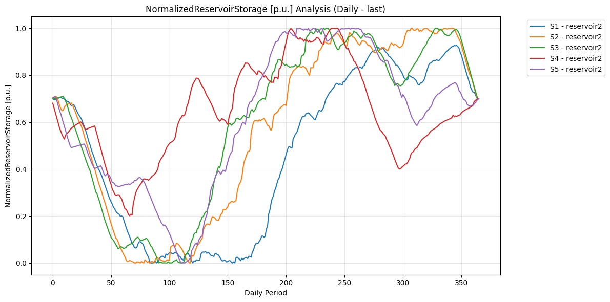
Many simple charts can be created in the first tab of the dashboard. Available variables include generation, inflows, marginal cost, market price, storage level, spillage and water value. As mentioned, the plotting function allows to select multiple generators and scenarios to plot. Additionally, the variable granularity and aggregation function can be changed.
In the following example, daily reservoir level is plotted for every scenario of ‘reservoir2’.
# General Trends Chart
plot_simple_variable(
    results,
    variable="NormalizedReservoirStorage [p.u.]",
    scenarios=("S1", "S2", "S3", "S4", "S5"),
    generators=("reservoir2",),
    granularity="Daily",
    agg_func="last",
)
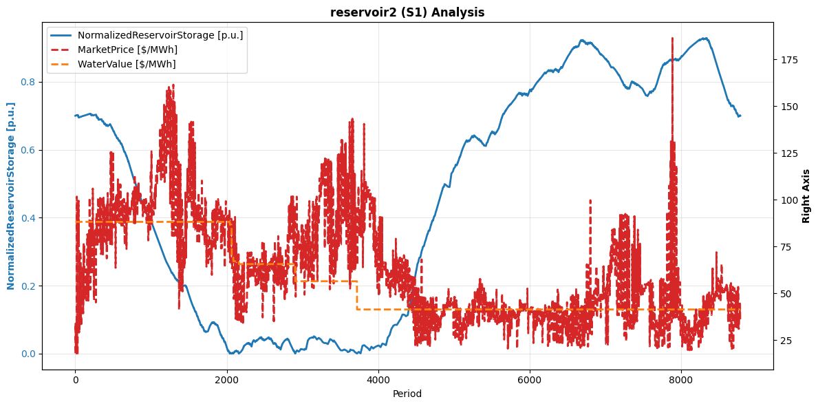
A more detailed plotting function is provided, in case multiple variables need to be compared. The function is designed specifically for the dams, including the same variables mentioned for the general trends charts. Furthermore, several variables can be selected at the same time for both axes, but constrained to only one reservoir and scenario.
In the example, storage level is compared with marginal price and water value for the first scenario of ‘reservoir2’.
plot_reservoir_analysis(
    results,
    reservoir="reservoir2",
    scenario="S1",
    left_vars=("NormalizedReservoirStorage [p.u.]",),
    right_vars=("MarketPrice [$/MWh]", "WaterValue [$/MWh]"),
)
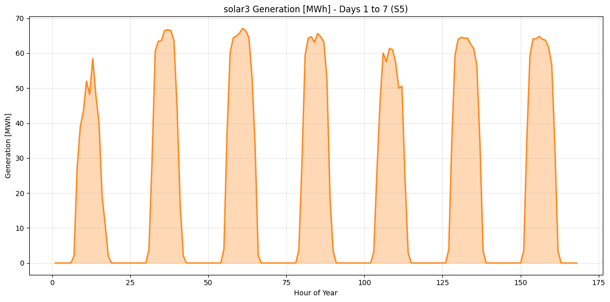
Finally, the using the last tab’s main plotting function, interesting hourly behaviour can be analysed. For instance, the following chart shows the solar generation of ‘solar3’ for the first week of the last scenario.
plot_variable_profile(
    results,
    variable="Generation [MWh]",
    generator="solar3",
    scenario="S5",
    day_range=(1, 7),
)
7. Analysis#
Several important conclusions can be drawn from the model and data explored in this notebook:
First of all, a single model run is not suited to handle uncertainty. This is due to the fact that the model can see all the future inflows and market price and assumes these variables will behave exactly as expected which is far from true. That’s one of the reasons why several scenarios were studied, but this will be further commented in a later section.
The chosen scenarios reflect the high volatility that inflows and market prices carry. In this same sense, the expected profit is also quite volatile. However, it’s very important to keep in mind that profit for a large generation firm comes from many sources (e.g. spot market, bilateral contracts, ancillary services, etc) and not only from the pool or exchange mechanism.
Using the dashboard above, the correct model behaviour can be confirmed. For instance, the model uses the reservoirs in the periods of higher prices and takes advantage of the wet season to fill them again, following an intuitive dam management policy that maximizes the income.
Renewable sources generation is also taken to full advantage respecting the physical and resource availability. This can be seen in the “Detailed Profiles” tab, where solar plants (if available in the scenario) follow a typical sun availability curve.
Thermal generation and ramps are also optimized by the model. Using them specially when market prices are higher than their costs (which would be the case in an economic dispatch, anyway).
Much valuable information can be drawn form the dual variables of the model. Water value is just one example of this. It is influenced by several variables such as the current and expected inflows, market price and reservoir storage level. In a bid-based market, this value (considering the different possible expected scenarios) can guide the bid price of the reservoir plants. Moreover, the model is also considering all the dams in the portfolio of the generation firms/
Another possible dual variable analysis that was not performed in this notebook is related to the maximum generation constraint. If maintenance schedule is included in this input, this value can be used for assessing different time windows alternatives betwwen different scenarios. Thus, periods where this variable is the lowest, should be conisdered and evaluated to program the maintenance.
7.1 Possible Modifications#
Several modifications can be made to the model to perform deeper analysis:
The presented model did not include battery storage systems. Adding them can find optimal patterns and complementarities between renewable intermittent sources and these assets.
Some binary variables can be added to explore unit-commitment and other types of constraints. However, this would make the model a MILP and performance can be drastically affected.
Incorporating some time reduction techniques can make the model suitable for longer planning horizons and additional integer constraints.
There are several options to approach uncertainty in this kind of application:
Sequential Decision Analytics (SDA): Reservoir management is intrisincally a sequential decision problem. Every day the firm decides over the use of the dams and forecasts also change over time. Designing an explicit policy and evaluating over the real behaviour of the variables can be of much benefit.
Stochastic Modeling: although several scenarios were evaluated they were not jointly optimized in a stochastic manner. Exploring this option can also be a way to model uncertainty but model performance can be affected depending on the number of scenarios considered.
The most important assumption in this model was the competitive market context. Without it, a large firm can, in fact, influence the market price. This can be explored through bi-level and non-linear models (see this for further information).
Finally, using
amplpyfunctionalities, the model can be easily incorporated in any decision process and flows, while keeping the model logic separated from other concerns such as data manipulation and results usability.